Lecture 03 – CS 189, Fall 2025
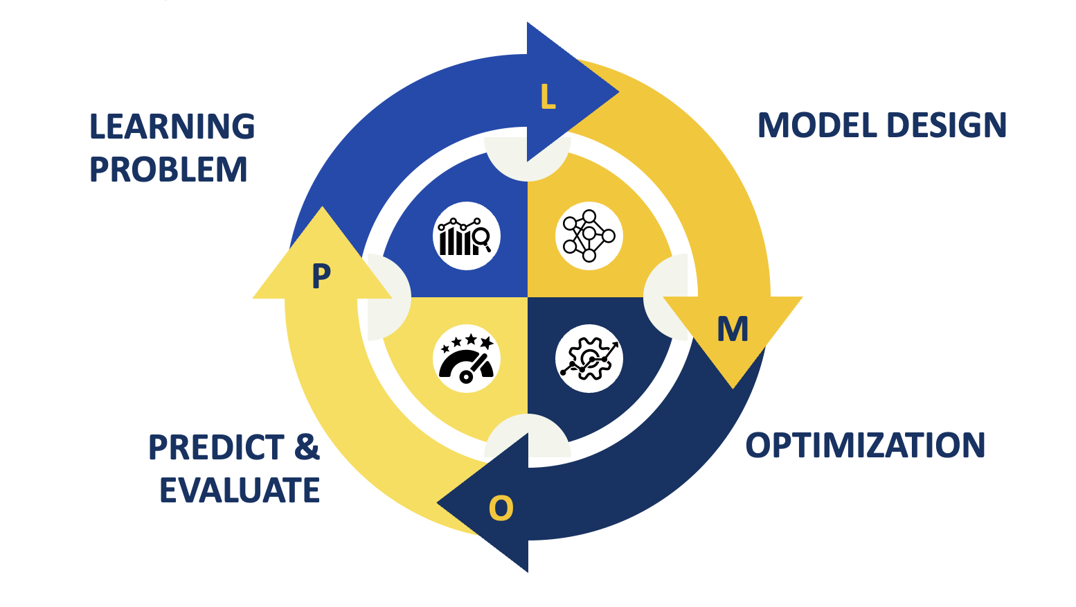
In this lecture, we will cover the basic machine learning lifecycle using a hands-on approach with scikit-learn. We will work through each stage of the machine learning lifecycle while also introducing standard machine learning tools and techniques. The machine learning lifecycle consists of four parts:
import numpy as np
import pandas as pd
import plotly.express as px
# Uncomment for HTML Export
import plotly.io as pio
pio.renderers.default = "notebook_connected"
The Learning Problem
Suppose we are launching a new fashion trading website where people can upload pictures of clothing they want to trade. We want to help posters identify the clothing in the images. Suppose we have some training data consisting of clothing pictures with labels describing the type of clothing (e.g., "dress", "shirt", "pants").
What data do we have?
- Labeled training examples.
What do we want to predict?
- The category label of the clothing in the images. We may want to predict other things as well.
How would we evaluate success?
- We likely want to measure our prediction accuracy.
- We may eventually want to improve accuracy on certain high-value classes.
Looking at the Data
A key step that is often overlooked in machine learning projects is understanding the data. This includes exploring the dataset, visualizing the data, and gaining insights into its structure and characteristics.
We will be using the Fashion-MNIST dataset, which is a (now) classic dataset with gray scale 28x28 images of articles of clothing.
Fashion-MNIST: a Novel Image Dataset for Benchmarking Machine Learning Algorithms. Han Xiao, Kashif Rasul, Roland Vollgraf. https://github.com/zalandoresearch/fashion-mnist
This is an alternative to the even more classic MNIST digits dataset, which contains images of handwritten digits.
The following block of code will download the Fashion-MNIST dataset and load it into memory.
# Fetch the Data
import torchvision
data = torchvision.datasets.FashionMNIST(root='data', train=True, download=True)

# Preprocess the data into numpy arrays
images = data.data.numpy().astype(float)
targets = data.targets.numpy() # integer encoding of class labels
class_dict = {i:class_name for i,class_name in enumerate(data.classes)}
labels = np.array([class_dict[t] for t in targets]) # raw class labels
n = len(images)

print("Loaded FashionMNIST dataset with {} samples.".format(n))
print("Classes: {}".format(class_dict))
print("Image shape: {}".format(images[0].shape))
print("Image dtype: {}".format(images[0].dtype))
print("Image 0:\n", images[0])
Loaded FashionMNIST dataset with 60000 samples.
Classes: {0: 'T-shirt/top', 1: 'Trouser', 2: 'Pullover', 3: 'Dress', 4: 'Coat', 5: 'Sandal', 6: 'Shirt', 7: 'Sneaker', 8: 'Bag', 9: 'Ankle boot'}
Image shape: (28, 28)
Image dtype: float64
Image 0:
 [[  0.   0.   0.   0.   0.   0.   0.   0.   0.   0.   0.   0.   0.   0.
    0.   0.   0.   0.   0.   0.   0.   0.   0.   0.   0.   0.   0.   0.]
 [  0.   0.   0.   0.   0.   0.   0.   0.   0.   0.   0.   0.   0.   0.
    0.   0.   0.   0.   0.   0.   0.   0.   0.   0.   0.   0.   0.   0.]
 [  0.   0.   0.   0.   0.   0.   0.   0.   0.   0.   0.   0.   0.   0.
    0.   0.   0.   0.   0.   0.   0.   0.   0.   0.   0.   0.   0.   0.]
 [  0.   0.   0.   0.   0.   0.   0.   0.   0.   0.   0.   0.   1.   0.
    0.  13.  73.   0.   0.   1.   4.   0.   0.   0.   0.   1.   1.   0.]
 [  0.   0.   0.   0.   0.   0.   0.   0.   0.   0.   0.   0.   3.   0.
   36. 136. 127.  62.  54.   0.   0.   0.   1.   3.   4.   0.   0.   3.]
 [  0.   0.   0.   0.   0.   0.   0.   0.   0.   0.   0.   0.   6.   0.
  102. 204. 176. 134. 144. 123.  23.   0.   0.   0.   0.  12.  10.   0.]
 [  0.   0.   0.   0.   0.   0.   0.   0.   0.   0.   0.   0.   0.   0.
  155. 236. 207. 178. 107. 156. 161. 109.  64.  23.  77. 130.  72.  15.]
 [  0.   0.   0.   0.   0.   0.   0.   0.   0.   0.   0.   1.   0.  69.
  207. 223. 218. 216. 216. 163. 127. 121. 122. 146. 141.  88. 172.  66.]
 [  0.   0.   0.   0.   0.   0.   0.   0.   0.   1.   1.   1.   0. 200.
  232. 232. 233. 229. 223. 223. 215. 213. 164. 127. 123. 196. 229.   0.]
 [  0.   0.   0.   0.   0.   0.   0.   0.   0.   0.   0.   0.   0. 183.
  225. 216. 223. 228. 235. 227. 224. 222. 224. 221. 223. 245. 173.   0.]
 [  0.   0.   0.   0.   0.   0.   0.   0.   0.   0.   0.   0.   0. 193.
  228. 218. 213. 198. 180. 212. 210. 211. 213. 223. 220. 243. 202.   0.]
 [  0.   0.   0.   0.   0.   0.   0.   0.   0.   1.   3.   0.  12. 219.
  220. 212. 218. 192. 169. 227. 208. 218. 224. 212. 226. 197. 209.  52.]
 [  0.   0.   0.   0.   0.   0.   0.   0.   0.   0.   6.   0.  99. 244.
  222. 220. 218. 203. 198. 221. 215. 213. 222. 220. 245. 119. 167.  56.]
 [  0.   0.   0.   0.   0.   0.   0.   0.   0.   4.   0.   0.  55. 236.
  228. 230. 228. 240. 232. 213. 218. 223. 234. 217. 217. 209.  92.   0.]
 [  0.   0.   1.   4.   6.   7.   2.   0.   0.   0.   0.   0. 237. 226.
  217. 223. 222. 219. 222. 221. 216. 223. 229. 215. 218. 255.  77.   0.]
 [  0.   3.   0.   0.   0.   0.   0.   0.   0.  62. 145. 204. 228. 207.
  213. 221. 218. 208. 211. 218. 224. 223. 219. 215. 224. 244. 159.   0.]
 [  0.   0.   0.   0.  18.  44.  82. 107. 189. 228. 220. 222. 217. 226.
  200. 205. 211. 230. 224. 234. 176. 188. 250. 248. 233. 238. 215.   0.]
 [  0.  57. 187. 208. 224. 221. 224. 208. 204. 214. 208. 209. 200. 159.
  245. 193. 206. 223. 255. 255. 221. 234. 221. 211. 220. 232. 246.   0.]
 [  3. 202. 228. 224. 221. 211. 211. 214. 205. 205. 205. 220. 240.  80.
  150. 255. 229. 221. 188. 154. 191. 210. 204. 209. 222. 228. 225.   0.]
 [ 98. 233. 198. 210. 222. 229. 229. 234. 249. 220. 194. 215. 217. 241.
   65.  73. 106. 117. 168. 219. 221. 215. 217. 223. 223. 224. 229.  29.]
 [ 75. 204. 212. 204. 193. 205. 211. 225. 216. 185. 197. 206. 198. 213.
  240. 195. 227. 245. 239. 223. 218. 212. 209. 222. 220. 221. 230.  67.]
 [ 48. 203. 183. 194. 213. 197. 185. 190. 194. 192. 202. 214. 219. 221.
  220. 236. 225. 216. 199. 206. 186. 181. 177. 172. 181. 205. 206. 115.]
 [  0. 122. 219. 193. 179. 171. 183. 196. 204. 210. 213. 207. 211. 210.
  200. 196. 194. 191. 195. 191. 198. 192. 176. 156. 167. 177. 210.  92.]
 [  0.   0.  74. 189. 212. 191. 175. 172. 175. 181. 185. 188. 189. 188.
  193. 198. 204. 209. 210. 210. 211. 188. 188. 194. 192. 216. 170.   0.]
 [  2.   0.   0.   0.  66. 200. 222. 237. 239. 242. 246. 243. 244. 221.
  220. 193. 191. 179. 182. 182. 181. 176. 166. 168.  99.  58.   0.   0.]
 [  0.   0.   0.   0.   0.   0.   0.  40.  61.  44.  72.  41.  35.   0.
    0.   0.   0.   0.   0.   0.   0.   0.   0.   0.   0.   0.   0.   0.]
 [  0.   0.   0.   0.   0.   0.   0.   0.   0.   0.   0.   0.   0.   0.
    0.   0.   0.   0.   0.   0.   0.   0.   0.   0.   0.   0.   0.   0.]
 [  0.   0.   0.   0.   0.   0.   0.   0.   0.   0.   0.   0.   0.   0.
    0.   0.   0.   0.   0.   0.   0.   0.   0.   0.   0.   0.   0.   0.]]
Understanding The Raw Features (Images)
How much data do we have?
images.shape
(60000, 28, 28)
The images are stored in a 60000 by 28 by 28 tensor. This means we have 60000 images, each of which is 28 pixels wide and 28 pixels tall. Each pixel is represented by a single value. What are those values?
counts, bins =  np.histogram(images, bins=255)
fig_pixels = px.bar(x=bins[1:], y=counts,  title="Pixel value distribution",
       log_y=True, labels={"x":"Pixel value", "y":"Count"})
fig_pixels
It is important to learn how to visualize and work with data. Here we use Plotly express to visualize the image. Note, I am using the 'gray_r' color map to visualize the images, which is a gray scale color map that is reversed (so that black is 1 and white is 0).
px.imshow(images[0], color_continuous_scale='gray_r')
The following snippet of code visualizes multiple images in a grid. You are not required to understand this code, but it is useful to know how to visualize images in Python.
def show_images(images, max_images=40, ncols=5, labels = None):
    """Visualize a subset of images from the dataset.
    Args:
        images (np.ndarray): Array of images to visualize [img,row,col].
        max_images (int): Maximum number of images to display.
        ncols (int): Number of columns in the grid.
        labels (np.ndarray, optional): Labels for the images, used for facet titles.
    Returns:
        plotly.graph_objects.Figure: A Plotly figure object containing the images.
    """
    n = min(images.shape[0], max_images) # number of images to show
    px_height = 220 # height of each image in pixels
    fig = px.imshow(images[:n, :, :], color_continuous_scale='gray_r',
                    facet_col = 0, facet_col_wrap=ncols,
                    height = px_height * int(np.ceil(n/ncols)))
    fig.update_layout(coloraxis_showscale=False)
    if labels is not None:
        # Extract the facet number and replace with the label.
        fig.for_each_annotation(lambda a: a.update(text=labels[int(a.text.split("=")[-1])]))
    return fig
show_images(images, 20, labels=labels)
Let's look at a few examples of each class. Here we use Pandas to group images by their labels and sample 2 for each class. You are not required to know Pandas (we won't test you on it), but it is a useful library for data manipulation and analysis and we will use it often in this course.
idx = (
    pd.DataFrame({"labels": labels})
      .groupby("labels", as_index=False)
      .sample(2)
      .index
      .to_numpy())
show_images(images[idx,:,:], labels=labels[idx])
Understanding the Labels
New let's examine the labels. Are they discrete? What is the distribution? Are there missing values or errors?
In the Fashion-MNIST dataset, each image is labeled with a class corresponding to a type of clothing. There are 10 classes in total.
However, it is also important to understand the distribution of labels in the dataset. This can help us identify potential issues such as class imbalance, where some classes have significantly more samples than others.
labels
array(['Ankle boot', 'T-shirt/top', 'T-shirt/top', ..., 'Dress',
       'T-shirt/top', 'Sandal'], shape=(60000,), dtype='<U11')
The labels are strings (discrete).
What is the distribution of labels?
px.histogram(labels, title="Label distribution")
There appear to be equal proportion of each type of clothing. We don't have any missing values since all labels are one of the 10 classes (no blank or "missing" label values).
Most real world datasets aren't this balanced or clean. In fact, it's common to see a long tail distribution, where a few classes are very common and many classes are rare.
Reviewing the Learning Setting
Having examined the data we can see that we have a large collection of pairs of features and categorical labels (with 10 classes). This is a supervised learning problem, where the goal is to learn a mapping from the input features (images) to the output labels (categories). Because the labels are discrete this is a classification problem.
It is also worth noting that because the input features are images this is also a computer vision problem. This means that when we get to the model development stage, we will need to consider techniques that are specifically designed for multi-class classification and in particular computer vision.
Return to Slides
Train-Test-Validation Split
We will split the dataset into a training set, a validation set, and a test set. The training set will be used to train the model, while the validation set will be used to tune the model's hyperparameters. The test set will be used to evaluate the model's performance.
Technically, the Fashion-MNIST dataset has a separate test set, but we will demonstrate how to split data in general.
# use sklearn to construct a train test split
from sklearn.model_selection import train_test_split
# Construct the train - test split
images_tr, images_te, labels_tr, labels_te = train_test_split(
    images, labels, test_size=0.2, random_state=42)

# Construct the train - validation split
images_tr, images_val, labels_tr, labels_val = train_test_split(
    images_tr, labels_tr, test_size=0.2, random_state=42)

print("images_tr shape:", images_tr.shape)
print("images_val shape:", images_val.shape)
print("images_te shape:", images_te.shape)
images_tr shape: (38400, 28, 28)
images_val shape: (9600, 28, 28)
images_te shape: (12000, 28, 28)
Return to Slides
Model Design
We have already loaded the Fashion-MNIST dataset in the previous section. Now, we will preprocess the data to make it suitable for training a classification model.
Feature Engineering
Feature Engineering is the process of transforming the raw features into a representation that can be used effectively by machine learning techniques. This will often involve transforming data into vector representations.
Naive Image Featurization
For this example we are working with low-resolution grayscale image data. Here we adopt a very simple featurization approach -- flatten the image. We will convert the 28x28 pixel images into 784-dimensional vectors.
images_tr.shape
(38400, 28, 28)
def flatten(images):
    return images.reshape(images.shape[0], -1)
X_tr = flatten(images_tr)
X_tr.shape
(38400, 784)
Standardization
Recall that the pixel intensities are from 0 to 255:
fig_pixels
Let's standardize the pixel intensities to have zero mean and unit variance.
Here we use the sklearn StandardScaler
from sklearn.preprocessing import StandardScaler

# 1. Initialize a StandardScaler object
image_scaler = StandardScaler()

# 2. Fit the scaler
image_scaler.fit(flatten(images_tr))
StandardScaler()In a Jupyter environment, please rerun this cell to show the HTML representation or trust the notebook.
On GitHub, the HTML representation is unable to render, please try loading this page with nbviewer.org.
Parameters
| copy | True | |
| with_mean | True | |
| with_std | True |
What do the mean and variance images tell us about the dataset?
display(px.imshow(image_scaler.mean_.reshape(28,28),
                  color_continuous_scale='gray_r', title="Mean image"))
display(px.imshow(image_scaler.var_.reshape(28,28),
                  color_continuous_scale='gray_r', title="Variance image"))
Let's create a generic featurization function that we can reuse for different datasets. Notice that this function uses the image_scaler that we fit to the training data.
def featurizer(images):
    flattened = flatten(images)
    return image_scaler.transform(flattened)

X_tr = featurizer(images_tr)
Our new images look similar to the original images but they have been standardized to have zero mean and unit variance. This should help improve the performance of our machine learning models.
show_images(X_tr.reshape(images_tr.shape), max_images=10, labels=labels_tr)
One-Hot Encoding
We don't need to one-hot encode the features in this dataset so we will briefly demonstrate on another dataset:
df = pd.DataFrame({"color": ["red", "green", "red", "blue", "blue", "yellow", ""]})
df
| color | |
|---|---|
| 0 | red |
| 1 | green |
| 2 | red |
| 3 | blue |
| 4 | blue |
| 5 | yellow |
| 6 |
from sklearn.preprocessing import OneHotEncoder
# 1. Initialize a OneHotEncoder object
ohe = OneHotEncoder()
# 2. Fit the encoder
ohe.fit(df[["color"]])
OneHotEncoder()In a Jupyter environment, please rerun this cell to show the HTML representation or trust the notebook.
On GitHub, the HTML representation is unable to render, please try loading this page with nbviewer.org.
Parameters
| categories | 'auto' | |
| drop | None | |
| sparse_output | True | |
| dtype | <class 'numpy.float64'> | |
| handle_unknown | 'error' | |
| min_frequency | None | |
| max_categories | None | |
| feature_name_combiner | 'concat' |
ohe.categories_
[array(['', 'blue', 'green', 'red', 'yellow'], dtype=object)]
ohe.transform(df[["color"]]).toarray()
ohe.categories_
[array(['', 'blue', 'green', 'red', 'yellow'], dtype=object)]
Bag of Words
We also don't need the bag-of-words representation for this dataset, but we will demonstrate it briefly using another dataset.
df['text'] = [
    "Red is a color.",
    "Green is for green food.",
    "Red reminds me of red food.",
    "Blue is my favorite color!",
    "Blue is for Cal!",
    "Yellow is also for Cal!",
    "I forgot to write something."
]
from sklearn.feature_extraction.text import CountVectorizer

# 1. Initialize a CountVectorizer object
vectorizer = CountVectorizer()

# 2. Fit the vectorizer
vectorizer.fit(df["text"])
CountVectorizer()In a Jupyter environment, please rerun this cell to show the HTML representation or trust the notebook.
On GitHub, the HTML representation is unable to render, please try loading this page with nbviewer.org.
Parameters
| input | 'content' | |
| encoding | 'utf-8' | |
| decode_error | 'strict' | |
| strip_accents | None | |
| lowercase | True | |
| preprocessor | None | |
| tokenizer | None | |
| stop_words | None | |
| token_pattern | '(?u)\\b\\w\\w+\\b' | |
| ngram_range | (1, ...) | |
| analyzer | 'word' | |
| max_df | 1.0 | |
| min_df | 1 | |
| max_features | None | |
| vocabulary | None | |
| binary | False | |
| dtype | <class 'numpy.int64'> |
pd.DataFrame(vectorizer.transform(df["text"]).toarray(),
             columns=vectorizer.get_feature_names_out())
| also | blue | cal | color | favorite | food | for | forgot | green | is | me | my | of | red | reminds | something | to | write | yellow | |
|---|---|---|---|---|---|---|---|---|---|---|---|---|---|---|---|---|---|---|---|
| 0 | 0 | 0 | 0 | 1 | 0 | 0 | 0 | 0 | 0 | 1 | 0 | 0 | 0 | 1 | 0 | 0 | 0 | 0 | 0 |
| 1 | 0 | 0 | 0 | 0 | 0 | 1 | 1 | 0 | 2 | 1 | 0 | 0 | 0 | 0 | 0 | 0 | 0 | 0 | 0 |
| 2 | 0 | 0 | 0 | 0 | 0 | 1 | 0 | 0 | 0 | 0 | 1 | 0 | 1 | 2 | 1 | 0 | 0 | 0 | 0 |
| 3 | 0 | 1 | 0 | 1 | 1 | 0 | 0 | 0 | 0 | 1 | 0 | 1 | 0 | 0 | 0 | 0 | 0 | 0 | 0 |
| 4 | 0 | 1 | 1 | 0 | 0 | 0 | 1 | 0 | 0 | 1 | 0 | 0 | 0 | 0 | 0 | 0 | 0 | 0 | 0 |
| 5 | 1 | 0 | 1 | 0 | 0 | 0 | 1 | 0 | 0 | 1 | 0 | 0 | 0 | 0 | 0 | 0 | 0 | 0 | 1 |
| 6 | 0 | 0 | 0 | 0 | 0 | 0 | 0 | 1 | 0 | 0 | 0 | 0 | 0 | 0 | 0 | 1 | 1 | 1 | 0 |
Return to Slides
Modeling and Optimization
In this section, we will go through the modeling process. We will focus on developing a classification model.
Training (Fitting) a Classifier
We will start with the most basic classifier, the logistic regression model, to demonstrate the classification workflow.
Logistic regression is a linear model that is commonly used for binary and multi-class classification tasks. It is also a good starting point for understanding more complex deep learning models that will be covered later in the course.
Here we use sklearn to fit a logistic regression model to the training data. The LogisticRegression class from sklearn.linear_model is used to create an instance of the model.
The fit method is called on the model instance, passing in the training data and labels. This trains the model to learn the relationship between the input features (flattened images) and the target labels (clothing categories). In scikit-learn, the fit method is used to train any model on the provided data.
from sklearn.linear_model import LogisticRegression

lr_model = LogisticRegression()
lr_model.fit(X=X_tr, y=labels_tr)
/opt/homebrew/Caskroom/mambaforge/base/envs/py_3_11/lib/python3.11/site-packages/sklearn/linear_model/_logistic.py:470: ConvergenceWarning:

lbfgs failed to converge after 100 iteration(s) (status=1):
STOP: TOTAL NO. OF ITERATIONS REACHED LIMIT

Increase the number of iterations to improve the convergence (max_iter=100).
You might also want to scale the data as shown in:
    https://scikit-learn.org/stable/modules/preprocessing.html
Please also refer to the documentation for alternative solver options:
    https://scikit-learn.org/stable/modules/linear_model.html#logistic-regression
LogisticRegression()In a Jupyter environment, please rerun this cell to show the HTML representation or trust the notebook.
On GitHub, the HTML representation is unable to render, please try loading this page with nbviewer.org.
Parameters
| penalty | 'l2' | |
| dual | False | |
| tol | 0.0001 | |
| C | 1.0 | |
| fit_intercept | True | |
| intercept_scaling | 1 | |
| class_weight | None | |
| random_state | None | |
| solver | 'lbfgs' | |
| max_iter | 100 | |
| multi_class | 'deprecated' | |
| verbose | 0 | |
| warm_start | False | |
| n_jobs | None | |
| l1_ratio | None |
Notice that we get a warning that:
plaintext
lbfgs failed to converge after 100 iteration(s) (status=1):
STOP: TOTAL NO. OF ITERATIONS REACHED LIMIT
This warning indicates that the optimization algorithm used by the logistic regression model did not converge to a solution within the default number of iterations. This can happen if the model is complex or if the data is not well-scaled.
We can change the optimization algorithm used by the logistic regression model. The default algorithm is lbfgs, which is a quasi-Newton method. Other options include newton-cg, sag, and saga. Each of these algorithms has its own strengths and weaknesses, and the choice of algorithm can affect the convergence speed and final performance of the model.
In this class, we will explore variations of stochastic gradient descent like saga. Let's try using the saga algorithm instead of lbfgs to see if it converges faster. Here we will also set the tol parameter since we don't want to wait.
lr_model = LogisticRegression(tol=0.05, solver='saga', random_state=42)
lr_model.fit(X=X_tr, y=labels_tr)
LogisticRegression(random_state=42, solver='saga', tol=0.05)In a Jupyter environment, please rerun this cell to show the HTML representation or trust the notebook.
On GitHub, the HTML representation is unable to render, please try loading this page with nbviewer.org.
Parameters
| penalty | 'l2' | |
| dual | False | |
| tol | 0.05 | |
| C | 1.0 | |
| fit_intercept | True | |
| intercept_scaling | 1 | |
| class_weight | None | |
| random_state | 42 | |
| solver | 'saga' | |
| max_iter | 100 | |
| multi_class | 'deprecated' | |
| verbose | 0 | |
| warm_start | False | |
| n_jobs | None | |
| l1_ratio | None |
Parameters
The parameters of a model are the internal variables that the model learns during the training process. For example, in logistic regression, the parameters are the weights assigned to each feature. These weights are adjusted during training to minimize the loss function, which measures how well the model's predictions match the actual labels.
print("model.coef_.shape:", lr_model.coef_.shape)
print("model.intercept_.shape:", lr_model.intercept_.shape)
print(lr_model.coef_)
print(lr_model.intercept_)
model.coef_.shape: (10, 784)
model.intercept_.shape: (10,)
[[ 9.90445492e-05 -6.36010321e-03 -3.85913757e-03 ...  1.49595978e-03
   4.32587736e-03  2.73064427e-03]
 [-1.89699677e-03  6.63981322e-03 -7.47402405e-03 ... -1.80362390e-02
  -1.84524048e-02 -1.52846533e-02]
 [-7.43264082e-04 -4.46484428e-03  1.60046019e-03 ...  5.50850058e-03
   1.38217724e-02  3.68772263e-03]
 ...
 [ 1.77951137e-04 -1.08447436e-03 -8.59128688e-04 ... -5.03797045e-03
  -1.78474348e-03 -2.49799352e-03]
 [-8.24675871e-03 -2.41366751e-03 -7.31344979e-03 ... -1.80925346e-02
  -1.21750176e-02 -1.40790500e-03]
 [-1.69500201e-04  7.44355526e-05 -5.08764217e-03 ... -5.67020645e-03
  -1.32036337e-03 -1.92847951e-03]]
[-0.03276315  0.01498156  0.02486191 -0.00368395  0.04477243 -0.06132416
  0.09267479 -0.03592529 -0.00330317 -0.04029096]
We can also visualize these coefficients. This can help us understand which pixels are most important for each class. We will learn more about this model in the future. (You don't have to understand these details now.)
coeffs = lr_model.coef_
show_images(coeffs.reshape(10, 28, 28), labels=lr_model.classes_)
Neural Networks
Neural networks are often the model of choice for image classification tasks. They can learn complex patterns in the data and often outperform simpler models like logistic regression. However, they also require the correct architecture and significant training data and computational resources.
Here we will try a simple neural network with two hidden layers.
from sklearn.neural_network import MLPClassifier
mlp = MLPClassifier(
    hidden_layer_sizes=(100, 50),
    max_iter=100, tol=1e-3, random_state=42)

mlp.fit(X=X_tr, y=labels_tr)
MLPClassifier(hidden_layer_sizes=(100, 50), max_iter=100, random_state=42,
              tol=0.001)
In a Jupyter environment, please rerun this cell to show the HTML representation or trust the notebook. On GitHub, the HTML representation is unable to render, please try loading this page with nbviewer.org.
Parameters
| hidden_layer_sizes | (100, ...) | |
| activation | 'relu' | |
| solver | 'adam' | |
| alpha | 0.0001 | |
| batch_size | 'auto' | |
| learning_rate | 'constant' | |
| learning_rate_init | 0.001 | |
| power_t | 0.5 | |
| max_iter | 100 | |
| shuffle | True | |
| random_state | 42 | |
| tol | 0.001 | |
| verbose | False | |
| warm_start | False | |
| momentum | 0.9 | |
| nesterovs_momentum | True | |
| early_stopping | False | |
| validation_fraction | 0.1 | |
| beta_1 | 0.9 | |
| beta_2 | 0.999 | |
| epsilon | 1e-08 | |
| n_iter_no_change | 10 | |
| max_fun | 15000 |
Hyperparameters
The hyperparameters are the arguments that are set before the training process begins. These include the choice of optimization algorithm, the learning rate, and the number of iterations, among others. Hyperparameters are typically tuned using techniques like cross-validation to find the best combination for a given dataset.
Confusingly these hyperparameters are often referred to as "parameters" in the context of machine learning libraries like sklearn. For example, the LogisticRegression class has hyperparameters like solver, C, and max_iter that can be adjusted to improve model performance.
lr_model
LogisticRegression(random_state=42, solver='saga', tol=0.05)In a Jupyter environment, please rerun this cell to show the HTML representation or trust the notebook.
On GitHub, the HTML representation is unable to render, please try loading this page with nbviewer.org.
Parameters
| penalty | 'l2' | |
| dual | False | |
| tol | 0.05 | |
| C | 1.0 | |
| fit_intercept | True | |
| intercept_scaling | 1 | |
| class_weight | None | |
| random_state | 42 | |
| solver | 'saga' | |
| max_iter | 100 | |
| multi_class | 'deprecated' | |
| verbose | 0 | |
| warm_start | False | |
| n_jobs | None | |
| l1_ratio | None |
To evaluate the model we will use the validation dataset.
X_val = featurizer(images_val)
Let's try tuning the regularization parameter C. To make this process more illustrative we will work with a smaller subset of the training data (n=1000). This will allow us to better demonstrate underfitting and overfitting and significantly speed up the training process.
n_small = 1000
X_tr_small = X_tr[:n_small,:]
labels_tr_small = labels_tr[:n_small]
In practice, we need to be careful when tuning regularization parameters against a sample of the data. In this case, more regularization is likely needed for smaller datasets to prevent overfitting.
from sklearn.metrics import log_loss

C_vals = np.logspace(-5, 1, 20)

logprob_tr = []
logprob_val = []
acc_tr = []
acc_val = []

for C in C_vals:
    print("starting training with C =", C)
    model = LogisticRegression(tol=1e-3, random_state=42, C=C)
    model.fit(X=X_tr_small, y=labels_tr_small)

    # compute the logprob accuracy
    logprob_tr.append(-log_loss(labels_tr_small, model.predict_proba(X_tr_small), labels=model.classes_))
    logprob_val.append(-log_loss(labels_val, model.predict_proba(X_val), labels=model.classes_))

    # compute the accuracy
    acc_tr.append(np.mean(model.predict(X_tr_small) == labels_tr_small))
    acc_val.append(np.mean(model.predict(X_val) == labels_val))
starting training with C = 1e-05
starting training with C = 2.06913808111479e-05
starting training with C = 4.281332398719396e-05
starting training with C = 8.858667904100833e-05
starting training with C = 0.00018329807108324357
starting training with C = 0.000379269019073225
starting training with C = 0.0007847599703514606
starting training with C = 0.001623776739188721
starting training with C = 0.003359818286283781
starting training with C = 0.0069519279617756054
starting training with C = 0.01438449888287663
starting training with C = 0.029763514416313162
starting training with C = 0.06158482110660261
starting training with C = 0.1274274985703132
starting training with C = 0.26366508987303555
starting training with C = 0.5455594781168515
starting training with C = 1.1288378916846884
starting training with C = 2.3357214690901213
starting training with C = 4.832930238571752
starting training with C = 10.0
df_logprob = pd.DataFrame({
    "C_val": C_vals,
    "Train": logprob_tr, "Validation": logprob_val,
}).set_index("C_val")

display(
    px.line(df_logprob,
        labels={"value": "Avg. Log Prob.", "C_val": "Reg. Parameter C"},
        title="LR Classifier Log Prog vs Reg. Parameter",
        markers=True,
        log_x=True,
        width=800, height=500)
)

df_acc = pd.DataFrame({
    "C_val": C_vals,
    "Train": acc_tr, "Validation": acc_val
}).set_index("C_val")

display(
    px.line(df_acc,
        labels={"value": "Accuracy", "C_val": "Reg. Parameter C"},
        title="LR Classifier Accuracy vs Reg. Parameter",
        markers=True,
        log_x=True,
        width=800, height=500
    )
)
Evaluating the Model
After training the model, we can use it to make predictions on new data. The predict method of the trained model is used to generate predictions based on the input features.
Let's return to our logistic regression model.
lr_model.predict(X_tr[:10,:])
array(['Ankle boot', 'Coat', 'Ankle boot', 'T-shirt/top', 'Pullover',
       'Ankle boot', 'Dress', 'T-shirt/top', 'Coat', 'Sandal'],
      dtype='<U11')
Do you agree with the predictions? Let's visualize the predictions on a few test images.
show_images(images_tr[:10,:].reshape(10, 28, 28),
            labels = lr_model.predict(X_tr[:10,:]))
Now let's see what the correct labels are for these images.
k = 10
tmp_labels = labels_tr[:k] + " (pred=" + lr_model.predict(X_tr[:k,:]) + ")"
show_images(images_tr[:k,:].reshape(k, 28, 28), labels=tmp_labels)
Predicting Probabilities
Many models can also provide probabilities for each class using the predict_proba method. This is useful for understanding the model's confidence in its predictions. In this class, we will often use a probabilistic framing, where we interpret the output of the model as probabilities of each class.
lr_model.predict_proba(X_tr[:5,:])
array([[9.51642010e-01, 1.25766964e-03, 8.94327054e-07, 3.11486837e-07,
        2.59469407e-07, 7.35306052e-03, 1.78581053e-07, 3.97435123e-02,
        5.22696365e-07, 1.58056694e-06],
       [1.05752334e-04, 2.47086595e-03, 8.32072100e-01, 3.44094506e-03,
        4.58904789e-02, 4.24209010e-05, 1.13951633e-01, 1.94167275e-05,
        1.55456636e-03, 4.51820449e-04],
       [9.30078717e-01, 1.40564685e-03, 1.91994009e-06, 6.84403412e-07,
        8.73522603e-07, 9.24863395e-03, 8.71969951e-07, 5.92557003e-02,
        1.75317539e-06, 5.19911487e-06],
       [2.05798117e-04, 2.21031435e-05, 6.61559787e-04, 2.37402967e-02,
        2.18046824e-02, 2.07214721e-05, 3.03973688e-02, 1.53740432e-04,
        9.18742226e-01, 4.25150290e-03],
       [2.23839377e-04, 9.60149725e-02, 1.08016253e-01, 2.85455925e-04,
        7.19252331e-01, 1.85483941e-03, 7.24570316e-02, 3.23939232e-04,
        1.53916187e-03, 3.21759981e-05]])
We can visualize these probabilities for the same images we predicted earlier.
k = 10
df = pd.DataFrame(lr_model.predict_proba(X_tr[:k,:]), columns=lr_model.classes_)
bars = px.bar(df, barmode='stack',orientation='v')
bars.update_layout(xaxis_tickmode='array', xaxis_tickvals=np.arange(k))
display(bars)
tmp_labels = labels_tr[:k] + " (pred=" + lr_model.predict(X_tr[:k,:]) + ") img: " + np.arange(k).astype(str)
show_images(images_tr[:k,:].reshape(k, 28, 28), labels=tmp_labels)
Accuracy Metrics and Test Performance
After training the model, we often want to evaluate the model. There are many ways to evaluate a model, and the best method depends on the task and the data. For classification tasks, we often use metrics like accuracy, precision, recall, and F1-score. Let's start with accuracy.
Accuracy is the simplest metric, which measures the proportion of correct predictions out of the total number of predictions.
Let's start by computing the accuracy of our model on the training set.
np.mean(lr_model.predict(X_tr) == labels_tr, axis=0)
np.float64(0.8488541666666667)
One of the issues with the training set is that the model may have overfit to the training data, meaning it performs well on the training set but poorly on unseen data. Intuitively, this is like practicing on a set of questions and then getting those same questions right on a test, but not being able to answer new questions that are similar but not identical.
To assess the model's performance on unseen data, we will evaluate it on the test set. Recall, the test set is a separate portion of the dataset that was not used during training.
X_te = featurizer(images_te)
np.mean(lr_model.predict(X_te) == labels_te, axis=0)
np.float64(0.84075)
from sklearn.metrics import accuracy_score

train_acc = accuracy_score(labels_tr, lr_model.predict(X_tr))
val_acc = accuracy_score(labels_val, lr_model.predict(X_val))
test_acc = accuracy_score(labels_te, lr_model.predict(X_te))

print("Train accuracy:", train_acc)
print("Validation accuracy:", val_acc)
print("Test accuracy:", test_acc)
Train accuracy: 0.8488541666666667
Validation accuracy: 0.849375
Test accuracy: 0.84075
The test accuracy is slightly lower than the training accuracy, which is expected. However, the difference is not too large, indicating that the model has not overfit significantly.
Is this accuracy good? What would a random guess yield?
A common way to evaluate a classification model is to compare its accuracy against a baseline. Perhaps the simplest baseline is random guessing, where we randomly assign a class to each image.
What accuracy does random guessing yield?
This would depend on the how frequently each class appears in the test dataset.
np.random.seed(42)
print("Model Accuracy:", np.mean(lr_model.predict(X_val) == labels_val, axis=0))
print("Random Guess Accuracy:",
      np.mean(np.random.choice(lr_model.classes_, size=len(labels_te)) == labels_te, axis=0))
Model Accuracy: 0.849375
Random Guess Accuracy: 0.10108333333333333
Does our model struggle with any particular class?
isWrong = lr_model.predict(X_val) != labels_val
# make a histogram with frequency of correct and incorrect predictions
fig = px.histogram(labels_val[isWrong], histnorm='percent')
fig.update_layout(xaxis_title="Label",
                  yaxis_title="Percentage of Incorrect Predictions")
fig.update_xaxes(categoryorder="total descending")
For classification tasks, we often want to look at more than just accuracy. We can use a confusion matrix to visualize the performance of the model across different classes. The confusion matrix shows the number of correct and incorrect predictions for each class.
from sklearn.metrics import confusion_matrix

fig = px.imshow(
    confusion_matrix(labels_val, lr_model.predict(X_val)),
    color_continuous_scale='Blues'
    )
fig.update_layout(
        xaxis_title="Predicted Label",
        yaxis_title="True Label",
        coloraxis_showscale=False,
        xaxis=dict(tickmode='array', tickvals=np.arange(len(model.classes_)), ticktext=model.classes_),
        yaxis=dict(tickmode='array', tickvals=np.arange(len(model.classes_)), ticktext=model.classes_)
    )
Last Thoughts
In the homework, you will have a chance to work with this data and use scikit-learn in more depth. We recommend reading the documentation and tutorial on the scikit-learn website as we go through the course. These provide a great resource for understanding the various functions and capabilities of the library as well as machine learning concepts.