import plotly.io as pio; pio.renderers.default = "notebook_connected"
Lecture 14 – CS 189, Fall 2025
import pandas as pd
import plotly.express as px
import plotly.graph_objects as go
from plotly import figure_factory as ff
from plotly.subplots import make_subplots
colors = px.colors.qualitative.Plotly
px.defaults.width = 800
# from ipywidgets import HBox
import numpy as np
Basics of Neural Networks
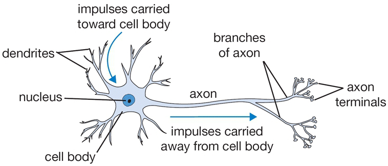
Neurons pass information from one to another using action potentials. They connect with one another at synapses, which are junctions between one neuron's axon and another's dendrite. Information flows from:
- The dendrites,
- To the cell body,
- Through the axons,
- To a synapse connecting the axon to the dendrite of the next neuron.
An Artificial Neuron is a mathematical function with the following elements:
- Input
- Weighted summation of inputs
- Processing unit of activation function
- Output
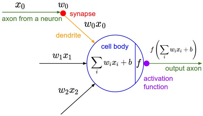
The mathematical equation for an artificial is as follows:
\begin{align} \hat{y} = f(\vec{\mathbf{\theta}} \cdot \vec{\mathbf{x}}) &= f\left(\sum_{i=0}^D w_i x_i\right) \\ &= f(w_0 + w_1 x_1 + ... + w_Dx_D). \end{align}
Assuming that function $f$ is the logistic or sigmoid function, the output of the neuron has a probability value ($0 \leq p \leq 1$). This probability value can then be used for a binary classification task where $p < 0.5$ is an indication of class $0$, and $p \geq 0.5$ assigns data to class 1. Re-writing the equation above with a sigmoid activation function would give us the following:
\begin{align} \hat{y} = σ(\vec{\mathbf{w}} \cdot \vec{\mathbf{x}}) &= \sigma\left(\sum_{i=0}^d w_i x_i\right) \\ &= σ(w_0 + w_1 x_1 + ... + w_Dx_D). \end{align}
The code below contains an implementation of AND, OR, and XOR gates. You will be able to generate data for each of the functions and add the desired noise level to the data. Familiarize yourself with the code and answer the following questions.
The Logic Gate Problem
We'll start by generating synthetic data for a logic gate (e.g., AND, OR, XOR) with Gaussian noise. This data will be used for training and testing the logistic regression model.
The function generate_data_with_noise allows customization of the number of samples, the logic gate, and the noise level.
# Function to generate a dataset with multiple samples per gate location
def generate_data_with_noise(num_samples = 500, gate = "AND", noise_level = 0.05):
"""
Generate multiple samples per logic gate configuration with added noise.
"""
if gate == 'AND':
base_X = np.array([[0, 0], [0, 1], [1, 0], [1, 1]])
base_t = np.array([0, 0, 0, 1])
elif gate == 'OR':
base_X = np.array([[0, 0], [0, 1], [1, 0], [1, 1]])
base_t = np.array([0, 1, 1, 1])
elif gate == 'XOR':
base_X = np.array([[0, 0], [0, 1], [1, 0], [1, 1]])
base_t = np.array([0, 1, 1, 0])
else:
raise ValueError("Gate must be 'AND', 'OR', or 'XOR'.")
# Repeat each base configuration to create multiple samples
X = np.repeat(base_X, num_samples // len(base_X), axis=0)
t = np.repeat(base_t, num_samples // len(base_t), axis=0)
# Add Gaussian noise to the inputs
X = X + np.random.normal(0, noise_level, X.shape)
# Shuffle the dataset to avoid ordered samples
indices = np.arange(X.shape[0])
np.random.shuffle(indices)
X = X[indices]
t = t[indices]
return X, t
In this lecture we will use interactive visualizations. These require a python environment so if you are viewing this notebook through the static HTML version you won't be able to use the interactive features.
from ipywidgets import interact, FloatSlider, Dropdown, Checkbox
import plotly.express as px
import plotly.graph_objects as go
X, t = generate_data_with_noise(500, 'AND', 0.05)
# Make an interactive plot
data_fig = go.FigureWidget()
data_fig.add_trace(go.Scatter(x=X[t == 0, 0], y=X[t == 0, 1], mode='markers',
marker=dict(color='red', opacity=0.7, size=7,
line=dict(width=1, color='DarkSlateGrey')),
name='0'))
data_fig.add_trace(go.Scatter(x=X[t == 1, 0], y=X[t == 1, 1], mode='markers',
marker=dict(color='blue', opacity=0.7, size=7,
line=dict(width=1, color='DarkSlateGrey')),
name='1'))
data_fig.update_layout(width=800, height=500,
xaxis_range=[-1, 2], yaxis_range=[-1, 2])
# The following code defines a set of interactive widgets (sliders)
# and binds them to an update function that will be run whenever
# a slider is changed.
@interact(num_samples=FloatSlider(min=100, max=1000, step=100, value=500, description='Samples'),
gate=Dropdown(options=['AND', 'OR', 'XOR'], value='AND', description='Gate'),
noise_level=FloatSlider(min=0.0, max=1.0, step=0.01, value=0.05, description='Noise Level'))
def update_data_plot(num_samples, gate, noise_level):
X, t = generate_data_with_noise(num_samples, gate, noise_level)
with data_fig.batch_update():
data_fig.data[0].x = X[t == 0, 0]
data_fig.data[0].y = X[t == 0, 1]
data_fig.data[1].x = X[t == 1, 0]
data_fig.data[1].y = X[t == 1, 1]
data_fig.update_layout(title=f"Dataset for {gate} Gate with Noise Level {noise_level}")
display(data_fig)
Solving with Logistic Regression
This section demonstrates how to perform logistic regression using the scikit-learn library. The dataset is divided into training and testing subsets using an 80%-20% ratio with the train_test_split function. A logistic regression model is instantiated and trained on the training dataset using the .fit() method. The model's performance is evaluated on both the training and testing data using the .score() method, which computes accuracy.
from sklearn.linear_model import LogisticRegression
from sklearn.model_selection import train_test_split
# Logistic Regression Using Scikit-learn
def perform_logistic_regression(X, t):
# Split the data
x_train, x_test, t_train, t_test = train_test_split(X, t, test_size=0.2, random_state=140)
# Train a logistic regression model
model = LogisticRegression().fit(x_train, t_train)
# Print training and testing scores
train_error = model.score(x_train, t_train)
test_error = model.score(x_test, t_test)
return model, train_error, test_error
We can plot a decision boundary or even a decision surface by plotting predictions on a regular grid of points. This is accomplished using the meshgrid function from numpy. We can then use the model to predict the class of each point on the grid and plot the results. This is a useful way to visualize the decision boundary of a classifier.
def plot_decision_boundary(model, x1_range, x2_range, num_points=100, probs=True):
# Generate a grid of points
x1, x2 = np.meshgrid(np.linspace(x1_range[0], x1_range[1], num_points),
np.linspace(x2_range[0], x2_range[1], num_points))
grid = np.c_[x1.ravel(), x2.ravel()]
# Get predictions for the grid
if probs:
preds = model.predict_proba(grid)[:,1].reshape(x1.shape)
else:
preds = model.predict(grid).reshape(x1.shape)
return go.Contour(x=x1[0], y=x2[:, 0], z=preds, colorscale=[[0, 'red'], [1, 'blue']],
opacity = 0.5, showscale=False)
Again we create an interactive visualization plot:
pred_fig = go.FigureWidget(data=data_fig.data, layout=data_fig.layout)
model, train_test, test_error = perform_logistic_regression(X, t)
boundary = plot_decision_boundary(model, [-1, 2], [-1, 2], probs=False)
pred_fig.add_trace(boundary)
@interact(num_samples=FloatSlider(min=100, max=1000, step=100, value=500, description='Samples'),
gate=Dropdown(options=['AND', 'OR', 'XOR'], value='AND', description='Gate'),
noise_level=FloatSlider(min=0.0, max=1.0, step=0.01, value=0.05, description='Noise Level'),
show_probs=Checkbox(value=False, description='Show Probabilities'))
def update_pred_fig(num_samples, gate, noise_level, show_probs):
np.random.seed(42)
X, y = generate_data_with_noise(num_samples, gate, noise_level)
model, train_error, test_error = perform_logistic_regression(X, y)
boundary = plot_decision_boundary(model, [-1, 2], [-1, 2], probs=show_probs)
with pred_fig.batch_update():
pred_fig.data[0].x = X[y == 0, 0]
pred_fig.data[0].y = X[y == 0, 1]
pred_fig.data[1].x = X[y == 1, 0]
pred_fig.data[1].y = X[y == 1, 1]
pred_fig.data[2].update(z=boundary.z)
title = f"Predictions for {gate} Gate with Noise Level {noise_level} (Train: {train_error:.2f}, Test: {test_error:.2f})"
pred_fig.update_layout(title=title)
display(pred_fig)
Let's focus on the XOR data and develop a neural network to classify it.
X, t = generate_data_with_noise(500, 'XOR', 0.15)
data = pd.DataFrame({'x1': X[:, 0], 'x2': X[:, 1], 't': t})
data_fig = go.Figure()
data_fig.add_trace(go.Scatter(x=X[t == 0, 0], y=X[t == 0, 1], mode='markers',
marker=dict(color='red', opacity=0.7, size=7,
line=dict(width=1, color='DarkSlateGrey')),
name='0'))
data_fig.add_trace(go.Scatter(x=X[t == 1, 0], y=X[t == 1, 1], mode='markers',
marker=dict(color='blue', opacity=0.7, size=7,
line=dict(width=1, color='DarkSlateGrey')),
name='1'))
data_fig.update_layout(width=600, height=500,
xaxis_range=[-1, 2], yaxis_range=[-1, 2])
Using PyTorch
PyTorch provides a flexible and efficient platform for building and training neural networks. PyTorch is known for its intuitive python centric approach to defining neural networks.
There are a few core concepts that are important to understand when using PyTorch:
- Tensors: Tensors are the fundamental data structure in PyTorch, similar to NumPy arrays but with additional capabilities for GPU acceleration. They can be used to represent inputs, outputs, and parameters of neural networks.
- DataSets and DataLoaders: PyTorch provides utilities to handle data loading and batching through
torch.utils.data.Datasetandtorch.utils.data.DataLoader. - nn.Module: This is the base class for all neural network modules in PyTorch. You can define your own models by subclassing
nn.Moduleand defining the layers and forward pass. - Optimizers: PyTorch provides various optimization algorithms (like SGD, Adam, etc.) in the
torch.optimmodule to update the model parameters based on the computed gradients. - Autograd: PyTorch's automatic differentiation library that tracks operations on tensors to compute gradients for backpropagation. (Focus of next lecture)
Importing Torch
When we import PyTorch (called torch for historical reasons), we typically import the main torch library and the torch.nn module, which contains classes and functions for building neural networks. We often alias torch.nn as nn for convenience.
import torch
import torch.nn as nn
import torch.nn.functional as F
One of the new features in torch is the torch._dynamo module, which is used to optimize the execution of PyTorch models. However, there are some known issues with torch._dynamo on certain hardware, such as Apple Silicon (M1/M2 chips). To avoid potential bugs or performance issues when running on Apple Silicon, we can disable torch._dynamo using the following command.
torch._dynamo.disable() # fixing a bug with apple silicon support
<torch._dynamo.eval_frame.DisableContext at 0x10fc809d0>
Tensors
Tensors are the fundamental data structure in PyTorch, similar to NumPy arrays but with additional capabilities for GPU acceleration. They can be used to represent inputs, outputs, and parameters of neural networks.
We can create tensors in various ways, such as from lists or NumPy arrays, or by using built-in functions to create tensors filled with zeros, ones, or random values. Here are some examples of creating tensors:
# Creating a tensor from a list
torch.tensor([[1, 2], [3, 4]], dtype=torch.float32)
tensor([[1., 2.],
[3., 4.]])
We can set the data type of a tensor using the dtype argument when creating it. Common data types include torch.float32, torch.int64, etc. Because we will work with hardware accelerators, it is important to be explicit about the data type of tensors.
torch.get_default_dtype()
torch.float32
Most accelerators will operate in float32 precision, so we will use torch.float32 for our input data and model parameters.
torch.zeros((2, 3)).dtype
torch.float32
Tensors generally inherit the data type of the input data, but it is good practice to be explicit about the data type when creating tensors, especially when working with hardware accelerators like GPUs or TPUs.
t = torch.tensor(data['t'])
print(t.dtype)
t = t.to(torch.float32)
print(t.dtype)
torch.int64 torch.float32
torch.mean(t, axis=0)
tensor(0.5000)
t = torch.tensor(data['t'], dtype=torch.float32)
print(t.dtype)
t
torch.float32
tensor([1., 0., 1., 1., 1., 1., 0., 1., 1., 0., 1., 1., 1., 1., 1., 0., 0., 0.,
0., 1., 0., 1., 1., 0., 0., 0., 0., 0., 0., 0., 1., 0., 1., 1., 0., 1.,
1., 1., 1., 0., 0., 0., 1., 0., 0., 0., 1., 0., 0., 0., 1., 0., 1., 0.,
1., 0., 1., 1., 0., 1., 0., 1., 0., 0., 1., 1., 0., 0., 0., 0., 0., 1.,
1., 1., 1., 0., 1., 0., 0., 1., 1., 0., 0., 0., 0., 1., 1., 0., 0., 0.,
0., 1., 1., 0., 1., 0., 1., 1., 0., 1., 0., 0., 0., 1., 0., 1., 0., 1.,
0., 0., 1., 0., 1., 1., 0., 1., 0., 0., 1., 0., 1., 0., 1., 1., 1., 0.,
0., 0., 0., 1., 0., 1., 1., 0., 1., 0., 1., 0., 0., 1., 1., 0., 1., 1.,
1., 1., 1., 1., 1., 0., 1., 1., 0., 1., 1., 1., 0., 1., 0., 0., 0., 0.,
0., 0., 0., 0., 1., 0., 0., 1., 0., 1., 0., 1., 1., 1., 0., 1., 0., 0.,
1., 1., 1., 1., 0., 0., 0., 0., 1., 1., 0., 0., 1., 1., 1., 1., 0., 0.,
1., 1., 1., 1., 0., 1., 1., 0., 1., 1., 1., 1., 0., 0., 1., 0., 0., 1.,
0., 1., 0., 1., 1., 0., 0., 1., 0., 1., 1., 1., 1., 0., 1., 0., 0., 1.,
0., 0., 1., 1., 1., 1., 0., 1., 0., 0., 0., 1., 0., 1., 0., 1., 1., 1.,
1., 1., 0., 0., 1., 1., 1., 1., 0., 0., 1., 1., 0., 1., 0., 0., 1., 1.,
1., 1., 0., 1., 0., 0., 1., 1., 1., 1., 1., 1., 0., 1., 1., 1., 1., 0.,
1., 0., 0., 1., 1., 0., 0., 0., 0., 0., 1., 1., 0., 1., 1., 0., 1., 0.,
1., 0., 1., 0., 1., 0., 1., 0., 0., 0., 0., 0., 1., 0., 0., 0., 1., 0.,
0., 0., 0., 0., 0., 0., 1., 1., 1., 0., 0., 0., 0., 0., 1., 1., 0., 0.,
0., 0., 0., 0., 1., 0., 0., 0., 1., 0., 1., 0., 0., 0., 1., 1., 1., 1.,
0., 1., 1., 1., 1., 0., 0., 1., 1., 1., 1., 0., 1., 1., 0., 0., 1., 0.,
1., 1., 1., 1., 0., 0., 0., 0., 0., 1., 1., 0., 1., 1., 0., 0., 0., 1.,
0., 1., 1., 1., 1., 0., 1., 0., 0., 1., 0., 0., 1., 1., 0., 0., 0., 1.,
0., 0., 1., 0., 1., 0., 0., 0., 1., 0., 1., 1., 1., 0., 0., 0., 0., 0.,
1., 0., 0., 1., 1., 1., 0., 1., 0., 1., 1., 1., 0., 0., 1., 0., 1., 0.,
1., 1., 1., 1., 1., 0., 0., 0., 1., 1., 0., 0., 0., 1., 1., 0., 0., 0.,
0., 0., 1., 0., 1., 1., 1., 0., 0., 1., 1., 0., 0., 1., 0., 0., 1., 1.,
1., 0., 0., 1., 1., 0., 0., 0., 0., 1., 1., 1., 1., 1.])
We can create data using other constructors, such as torch.zeros, torch.ones, and torch.rand:
# Creating a tensor filled with zeros
torch.zeros((2, 3))
tensor([[0., 0., 0.],
[0., 0., 0.]])
# Creating a tensor filled with ones
torch.ones((3, 2))
tensor([[1., 1.],
[1., 1.],
[1., 1.]])
# Creating a tensor with random values
torch.rand((2, 2))
tensor([[0.2994, 0.3895],
[0.8544, 0.9181]])
generator = torch.Generator().manual_seed(42)
torch.rand((2, 2), generator=generator)
tensor([[0.8823, 0.9150],
[0.3829, 0.9593]])
We can manipulate tensors using various operations, such as addition, multiplication, and matrix multiplication. Here are some examples of tensor operations:
x = torch.tensor([[1, 2], [3, 4]], dtype=torch.float32)
t = torch.tensor([[5, 6], [7, 8]], dtype=torch.float32)
x @ t
tensor([[19., 22.],
[43., 50.]])
torch.mean(x, axis=1)
tensor([1.5000, 3.5000])
We can slice and index tensors similarly to NumPy arrays. Here are some examples of slicing and indexing tensors:
x[0]
tensor([1., 2.])
x[:,1]
tensor([2., 4.])
Moving between numpy arrays and torch tensors is easy. Here are some examples:
x.numpy()
array([[1., 2.],
[3., 4.]], dtype=float32)
x[1,1]
tensor(4.)
x[1,1].item()
4.0
torch.tensor(np.random.randn(2,3))
tensor([[ 0.3546, -0.0450, -1.0173],
[ 0.0324, 0.7491, 1.1088]], dtype=torch.float64)
x[1,:]
tensor([3., 4.])
Working with Hardware Accelerators
Pytorch allows us to easily work with hardware accelerators like GPUs. This is particularly useful for training large neural networks, as it can significantly speed up the computations.
if torch.accelerator.is_available():
device = torch.accelerator.current_accelerator()
else:
device = "cpu"
print("Congratulations! You have access to a", device, "device.")
Congratulations! You have access to a mps device.
We can move tensors to the appropriate device (CPU or GPU) using the .to(device) method. Here is an example of how to check for available hardware accelerators and set the default device accordingly:
generator = torch.Generator(device=device).manual_seed(42)
x = torch.randn(3,2, device=device, generator=generator)
x
tensor([[ 0.9047, 0.2227],
[ 0.1460, 0.7360],
[-0.4142, -0.1106]], device='mps:0')
We can also move back to the CPU if needed using the same .to("cpu") method.
x.to("cpu")
tensor([[ 0.9047, 0.2227],
[ 0.1460, 0.7360],
[-0.4142, -0.1106]])
x.cpu()
tensor([[ 0.9047, 0.2227],
[ 0.1460, 0.7360],
[-0.4142, -0.1106]])
You cannot perform numpy operations on tensors that are on a device. You must first move them back to the CPU using the .cpu() method.
x.cpu().numpy()
array([[ 0.9046778 , 0.22267687],
[ 0.1460281 , 0.7360334 ],
[-0.41420847, -0.11061821]], dtype=float32)
Here is a simple function to convert tensors to numpy arrays safely:
def to_numpy(tensor):
"""Convert a PyTorch tensor to a NumPy array."""
return tensor.cpu().numpy()
You can also set the default device for all tensors using torch.set_default_device(device). This way, any new tensor created will automatically be on the specified device. This is particularly useful when you want to ensure that all tensors are on the same device without having to specify the device each time you create a tensor.
torch.set_default_device(device)
Let's convert our synthetic xor data to a tensor and move it to the appropriate device:
x = torch.tensor(data[['x1','x2']].values, dtype=torch.float32, device=device)
t = torch.tensor(data['t'].values, dtype=torch.float32, device=device)
Datasets
PyTorch uses Datasets to represent the collections of training data. PyTorch provides a convenient way to create datasets using the torch.utils.data.TensorDataset class. This class allows us to combine our input features and labels into a single dataset object, which can then be used for training and evaluation.
from torch.utils.data import TensorDataset
dataset = TensorDataset(
torch.tensor(data[['x1','x2']].values, dtype=torch.float32),
torch.tensor(data['t'].values, dtype=torch.float32))
dataset
<torch.utils.data.dataset.TensorDataset at 0x114fc6050>
We can access the dataset entries
x, t = dataset[1:5]
x, t
(tensor([[ 0.0430, -0.0173],
[ 0.0534, 1.0073],
[ 0.9215, -0.0056],
[-0.0116, 1.0952]], device='mps:0'),
tensor([0., 1., 1., 1.], device='mps:0'))
len(dataset)
500
There are useful utilities to manipulate datasets, such as constructing the train-validation split.
from torch.utils.data import random_split
generator = torch.Generator(device=device).manual_seed(189)
train_data, validation_data = random_split(
dataset, [.8, .2],
generator=generator)
len(train_data), len(validation_data)
(400, 100)
Here we make a dataset builder function:
def make_datasets_from_numpy(x, t, split_ratio=0.8, seed=189):
"""Create training and test datasets from numpy data arrays."""
from torch.utils.data import random_split, TensorDataset
data = TensorDataset(
torch.tensor(x, dtype=torch.float32, device=device),
torch.tensor(t, dtype=torch.long, device=device),
)
generator = torch.Generator(device=device).manual_seed(seed)
train_data, test_data = random_split(
data, [split_ratio, 1 - split_ratio],
generator=generator)
return train_data, test_data
training_data, validation_data = make_datasets_from_numpy(
data[['x1','x2']].values, data['t'].values)
(x, t) = training_data[:]
x, t
(tensor([[ 9.5965e-01, 1.2348e+00],
[ 1.2222e+00, -7.1787e-02],
[ 6.9757e-02, 2.4998e-02],
[ 1.4059e-01, 2.2820e-01],
[ 9.8363e-01, 9.2671e-01],
[ 1.7397e-01, 9.4346e-01],
[ 9.7220e-01, 7.3884e-01],
[ 3.5896e-02, 1.2144e+00],
[-3.7726e-01, 4.2304e-03],
[ 5.4969e-02, -3.8543e-02],
[ 1.0330e+00, 8.0109e-01],
[ 8.7099e-01, 8.3526e-02],
[ 5.8298e-03, 1.0231e+00],
[ 6.3777e-02, 5.0349e-02],
[ 9.1572e-01, -1.9929e-01],
[-4.3139e-02, -1.4124e-01],
[-2.0077e-03, 8.0463e-02],
[ 1.6373e-01, 7.9952e-02],
[ 1.3701e+00, 8.5115e-01],
[ 9.8732e-01, 8.9916e-01],
[ 1.8737e-01, -4.5014e-02],
[-2.9537e-01, -3.2738e-02],
[ 1.2504e+00, 1.3652e+00],
[-1.8881e-01, 8.4863e-01],
[ 7.8719e-01, 1.0320e+00],
[ 1.0475e+00, 2.8514e-01],
[ 1.1672e+00, 1.1671e+00],
[ 9.7948e-01, 1.1635e+00],
[ 6.8899e-01, 9.3564e-01],
[-8.2604e-02, 1.1416e+00],
[-1.4151e-01, 8.3141e-01],
[-1.0546e-01, 6.5095e-02],
[ 1.2276e+00, 2.5430e-01],
[ 5.8483e-02, 8.8414e-01],
[ 9.5597e-01, 1.6970e-02],
[ 5.4795e-02, 2.1031e-01],
[ 1.0227e+00, 1.0038e+00],
[ 5.5085e-02, 1.2382e+00],
[-2.0068e-01, 1.0827e+00],
[-1.9092e-01, 2.0181e-01],
[ 2.4592e-01, -1.4894e-02],
[ 1.0972e+00, 1.1134e+00],
[ 1.1360e+00, -3.2325e-02],
[ 9.7471e-01, -9.7153e-02],
[ 1.2651e-01, 1.0743e+00],
[ 8.9946e-01, 4.0111e-02],
[ 7.6761e-02, 8.7170e-01],
[ 1.1615e+00, 8.8853e-02],
[ 4.7256e-02, -2.4957e-02],
[ 1.0394e+00, 1.5768e-01],
[-1.9116e-01, 9.3911e-02],
[ 8.3279e-01, 1.4651e-02],
[ 1.0207e+00, 9.4901e-01],
[ 1.6014e-01, 1.1272e+00],
[ 8.5927e-01, 2.1279e-02],
[-5.0397e-02, 1.0649e+00],
[-2.4359e-01, 1.0242e+00],
[ 8.6450e-01, 9.8662e-01],
[-2.6142e-01, -7.4430e-04],
[ 9.0711e-01, 4.6968e-02],
[ 1.1906e+00, 1.0946e+00],
[-3.5496e-02, 1.1725e+00],
[ 1.0069e+00, -7.6279e-03],
[-1.6645e-01, 8.7403e-01],
[ 1.0277e+00, 8.4206e-01],
[ 5.5874e-02, 2.3987e-01],
[ 1.1389e+00, 9.2896e-01],
[ 9.6731e-01, 8.3340e-01],
[ 8.2271e-01, 1.2532e-01],
[ 1.2980e-01, 1.1461e-01],
[ 9.7953e-01, -2.4268e-01],
[ 3.5364e-02, -2.7375e-03],
[ 9.6922e-01, 1.2868e-01],
[-2.4846e-01, 1.8847e-01],
[ 5.6126e-01, 1.1872e+00],
[-1.4658e-02, 1.2118e+00],
[ 9.0126e-01, 9.4094e-01],
[ 8.7114e-01, 1.1793e+00],
[-2.0404e-03, 1.2186e+00],
[ 8.1906e-01, 8.0796e-01],
[-5.9097e-02, -6.1774e-02],
[ 1.8661e-01, -3.3047e-01],
[ 1.2134e-01, -1.0657e-01],
[ 8.4652e-01, -1.1916e-01],
[-2.9909e-01, 1.8275e-01],
[ 1.0586e+00, 1.1894e-01],
[ 6.1142e-01, 9.9266e-01],
[ 1.1542e+00, 1.0197e+00],
[ 1.5244e+00, 7.8049e-01],
[ 4.8777e-02, -2.5009e-02],
[ 1.1431e+00, 9.9329e-01],
[-5.2348e-02, 9.4674e-01],
[ 2.4401e-02, -1.2845e-01],
[ 1.3385e+00, 9.5389e-01],
[ 6.7104e-02, 8.1791e-01],
[-8.0617e-03, 1.1219e+00],
[-5.2497e-02, 8.2421e-02],
[ 1.1181e-01, 8.6711e-01],
[ 2.4092e-01, 2.3437e-01],
[ 1.1702e+00, -1.2186e-01],
[ 5.2693e-02, 1.2535e+00],
[ 1.0329e+00, 1.1934e+00],
[ 9.4345e-01, 8.6367e-02],
[ 1.7953e-01, 1.2462e-02],
[-9.1633e-02, 1.7918e-01],
[-8.9155e-02, 9.7115e-01],
[ 8.9497e-02, 1.1543e-01],
[ 9.1561e-01, 3.4174e-01],
[ 3.6280e-02, -1.4543e-01],
[-8.1023e-02, 4.7108e-02],
[ 6.2435e-02, 1.6143e-01],
[-8.0653e-02, 4.5517e-02],
[ 1.0021e+00, 2.3428e-02],
[-2.1668e-01, -2.4919e-01],
[ 5.5128e-02, 9.0757e-01],
[ 8.6360e-01, 4.3314e-03],
[ 1.0127e+00, -1.2698e-02],
[ 1.2588e+00, 1.0081e-01],
[ 5.1392e-02, 1.0330e+00],
[-7.4065e-03, 9.5456e-01],
[ 1.0423e+00, 1.2353e+00],
[-1.1374e-02, 1.1313e+00],
[ 1.0242e+00, -5.9220e-02],
[ 1.2903e-01, -3.1943e-01],
[ 3.2993e-01, 1.0798e+00],
[ 9.6886e-01, -2.6250e-01],
[ 1.1249e+00, 1.0378e+00],
[-1.2122e-01, 8.9268e-01],
[ 1.1607e-01, 1.6833e-01],
[ 1.2130e+00, 9.1979e-01],
[ 5.3644e-02, 8.7440e-01],
[-1.7972e-01, 8.0903e-01],
[ 1.2234e-02, 1.1960e+00],
[ 8.7420e-01, 1.0604e+00],
[ 7.0998e-01, 1.2533e+00],
[ 8.1376e-01, 2.4940e-02],
[-4.1134e-02, 8.5010e-01],
[ 7.2395e-01, 1.2415e+00],
[ 7.3595e-02, -1.5419e-01],
[-6.1713e-02, 1.0793e+00],
[ 8.7828e-01, 5.8308e-02],
[ 6.7006e-01, -2.5687e-01],
[ 1.1910e+00, -7.4740e-02],
[ 1.1707e+00, 1.0524e+00],
[ 9.2147e-01, -5.6035e-03],
[ 8.0681e-01, -3.9471e-01],
[-7.2030e-02, 1.1071e+00],
[-7.4625e-02, 8.9672e-01],
[ 9.3783e-01, 9.0871e-01],
[-3.5487e-02, -5.9459e-02],
[ 1.1014e-01, -1.4901e-01],
[ 1.0303e+00, -1.1669e-01],
[-1.2639e-01, 1.1505e+00],
[ 1.0490e+00, 2.4435e-01],
[ 4.1506e-02, 1.1098e+00],
[ 8.9419e-01, 1.0093e+00],
[ 3.0298e-01, 7.2544e-01],
[-9.8345e-02, 1.0223e+00],
[ 1.0311e+00, 1.1590e+00],
[ 1.0298e-01, -3.3198e-01],
[-5.8439e-02, 8.3075e-02],
[-8.9755e-02, 1.2462e+00],
[ 8.5057e-01, 9.9077e-01],
[-9.0316e-02, 4.1005e-02],
[ 9.7223e-01, -2.3892e-01],
[ 9.6386e-01, 7.6815e-01],
[-1.4902e-01, 8.6910e-02],
[ 1.0259e+00, 9.3359e-01],
[-1.8477e-02, 1.1679e+00],
[-4.5337e-02, 1.0335e+00],
[ 1.8969e-01, 9.3053e-01],
[-7.5472e-02, 1.2166e+00],
[ 9.5136e-02, 7.1293e-02],
[ 6.0643e-01, -1.8310e-01],
[ 2.3168e-01, 1.4178e-01],
[ 6.1480e-03, 1.2442e-01],
[ 1.2637e-01, 9.4559e-01],
[ 1.0897e+00, -1.2741e-01],
[-1.0991e-01, -1.0525e-01],
[ 1.1443e+00, -1.6911e-01],
[-1.3607e-01, 1.1585e+00],
[ 9.5560e-01, 1.6254e-01],
[ 3.0937e-02, -1.8077e-01],
[-7.6997e-02, 1.0042e+00],
[ 1.0438e+00, 9.7252e-01],
[-2.3719e-01, 5.4165e-03],
[ 1.1401e+00, 9.5120e-01],
[ 2.2172e-01, -7.4355e-02],
[ 1.0341e+00, -3.1739e-01],
[-1.6717e-01, -5.5347e-02],
[-2.2991e-01, 1.5494e-01],
[ 1.0090e+00, 8.0151e-01],
[-1.9403e-01, 1.6169e-01],
[ 1.1349e+00, 1.1117e+00],
[ 7.4672e-01, 1.7132e-01],
[ 1.1091e+00, -1.0113e-01],
[-1.8462e-01, -3.9051e-02],
[ 1.4228e-01, 5.2279e-03],
[-1.4231e-01, -3.2428e-01],
[ 3.6753e-02, -2.9614e-02],
[ 1.1923e+00, 1.7530e-02],
[-4.6282e-02, 1.0304e-01],
[-1.9244e-01, 8.6172e-01],
[ 4.3570e-03, 1.6130e-01],
[ 1.3164e+00, 1.1769e-01],
[ 9.9725e-01, 5.9587e-02],
[ 1.0345e+00, 1.2220e+00],
[-1.2050e-01, 6.8050e-01],
[ 8.7301e-01, 1.1097e+00],
[-3.6509e-01, 2.7865e-02],
[ 1.9651e-01, 5.8746e-03],
[ 1.0251e-01, 9.1088e-01],
[ 1.2824e+00, 1.1179e+00],
[ 8.7100e-01, 8.4550e-01],
[ 7.0500e-02, 1.2872e+00],
[-1.6039e-01, 7.0952e-01],
[-3.5742e-02, 8.4794e-01],
[-1.1969e-01, -2.1710e-02],
[ 2.9158e-01, 7.5656e-01],
[ 3.2879e-01, 1.0210e-01],
[ 1.9360e-02, 9.2665e-01],
[-4.0712e-01, 8.8008e-01],
[ 1.9059e-01, 8.9390e-01],
[ 1.0840e+00, 9.0766e-01],
[ 1.6067e-01, 8.9078e-01],
[ 1.4010e+00, 1.4353e-01],
[ 7.4664e-01, 8.9210e-01],
[ 1.6396e-01, 8.6305e-02],
[ 1.0557e+00, 1.1730e+00],
[ 2.0341e-01, 8.8082e-01],
[ 7.8776e-01, -3.8897e-01],
[ 1.1475e+00, 9.5369e-01],
[ 3.1934e-01, 1.0330e-01],
[-1.7351e-01, -2.3068e-01],
[-1.0960e-02, -1.6005e-01],
[ 1.0692e+00, 1.1355e+00],
[ 1.1032e+00, 6.2950e-02],
[ 1.0447e+00, 4.3310e-02],
[ 1.8161e-01, 9.2856e-02],
[ 1.0994e+00, 8.7007e-01],
[ 1.1938e+00, 1.2023e+00],
[-3.0128e-02, 9.7875e-01],
[ 8.9064e-01, 1.1572e+00],
[ 8.1370e-02, 1.1882e+00],
[ 1.3050e+00, 1.2803e-02],
[-1.0254e-01, 1.0643e-01],
[ 1.0805e+00, 4.6041e-02],
[ 9.9928e-01, 1.1160e+00],
[ 9.6086e-01, 8.0683e-01],
[ 1.0947e+00, -9.8112e-02],
[-4.3621e-02, -6.1173e-02],
[ 1.1174e+00, 7.8403e-01],
[-1.3165e-01, 1.1174e+00],
[ 8.7451e-01, 1.2375e+00],
[ 8.7664e-01, 1.1975e+00],
[ 9.4615e-01, 3.4819e-02],
[-8.3592e-02, 8.4039e-01],
[ 1.6872e-01, -1.1991e-01],
[ 1.1631e+00, 1.0273e+00],
[ 5.8045e-02, 2.0515e-01],
[-2.2625e-02, 9.6445e-01],
[ 8.6718e-02, -7.8360e-02],
[ 1.1210e+00, 3.0907e-02],
[ 9.7472e-01, 1.0299e+00],
[-2.5503e-01, 1.0792e+00],
[ 1.0282e+00, 7.6094e-01],
[-8.4390e-02, -9.0238e-02],
[ 1.0083e+00, 3.8203e-01],
[ 1.0161e+00, 1.7950e-01],
[ 9.9220e-01, 2.4623e-01],
[ 9.1818e-01, -7.3550e-03],
[ 1.1557e+00, 1.2955e-02],
[-2.7524e-03, 1.9677e-01],
[-8.7396e-02, 9.7431e-01],
[ 9.0701e-01, 1.3611e+00],
[-6.4880e-02, 1.9906e-01],
[-1.9916e-01, 9.9763e-01],
[ 2.5305e-01, 1.2511e+00],
[ 1.0015e+00, 1.0277e+00],
[ 8.3154e-01, 9.5137e-01],
[ 9.9391e-01, -1.7680e-01],
[ 8.8166e-01, -7.0624e-02],
[ 9.7447e-01, 8.0289e-01],
[-7.1550e-02, 1.1000e+00],
[ 1.3360e+00, 6.9011e-02],
[ 1.2751e-01, 1.1314e+00],
[ 1.1936e-01, 1.0928e+00],
[ 8.0979e-01, 1.8499e-02],
[ 1.0047e+00, 1.0935e+00],
[ 7.4189e-02, -1.7499e-02],
[-2.3413e-01, 7.8580e-01],
[ 6.6900e-02, 8.9451e-01],
[ 1.1434e+00, 1.2879e+00],
[ 9.5813e-01, 1.5416e-01],
[ 1.2309e+00, -1.0442e-01],
[-1.3316e-01, 1.0172e+00],
[-1.1547e-01, -8.4068e-02],
[ 1.1593e+00, -7.0115e-02],
[ 1.2578e+00, -4.3066e-02],
[-6.8821e-03, 3.0645e-01],
[ 1.1627e+00, 7.3491e-02],
[ 1.1814e+00, -2.1593e-01],
[-1.4885e-01, 5.7883e-02],
[ 2.3314e-02, 3.6986e-01],
[ 9.6737e-01, 7.7665e-01],
[ 7.0590e-02, 1.0952e-01],
[ 8.4892e-01, 1.0252e+00],
[ 8.5536e-01, 1.1404e+00],
[-4.7636e-02, 8.9868e-01],
[ 1.0843e+00, 1.0626e+00],
[-1.0370e-01, 6.6646e-01],
[ 3.4727e-02, -5.0274e-01],
[ 8.3732e-01, 8.4756e-01],
[-6.3630e-02, -1.4102e-01],
[ 7.8944e-01, -2.1797e-01],
[ 9.0887e-01, 1.1141e+00],
[-6.5117e-02, -8.1567e-02],
[ 1.0597e+00, 1.0237e+00],
[-2.2438e-01, 1.3232e-01],
[ 3.0626e-01, 1.1413e+00],
[-1.2347e-01, 9.7537e-01],
[ 8.7017e-01, 3.1253e-02],
[ 1.0780e+00, 1.2915e+00],
[ 9.3094e-01, 1.1297e+00],
[ 8.3475e-01, 9.5444e-02],
[ 1.2673e+00, -1.5978e-01],
[ 1.2425e+00, 8.3519e-01],
[ 7.0434e-02, 8.4902e-01],
[ 8.7012e-01, 8.9211e-01],
[ 1.0786e+00, 4.0713e-02],
[ 1.1256e+00, 1.1960e+00],
[ 1.1444e+00, 3.5456e-01],
[ 5.5959e-02, 3.0029e-01],
[ 1.1997e+00, 1.1427e-01],
[ 1.1598e+00, -9.5151e-02],
[ 8.0997e-01, 6.6389e-03],
[ 4.6874e-02, 4.7900e-02],
[ 9.2651e-02, 1.1047e+00],
[ 1.0285e+00, 1.1352e+00],
[ 1.5163e-01, -1.9577e-02],
[-7.7687e-02, 1.0362e+00],
[ 8.7461e-01, -1.5432e-02],
[ 1.1503e+00, 1.0776e+00],
[ 1.0487e+00, -5.3687e-02],
[ 1.1821e+00, -1.3020e-01],
[ 9.6673e-01, 1.0116e-01],
[ 1.0865e+00, -3.5876e-01],
[-1.5351e-01, 4.5258e-02],
[ 1.1698e+00, 3.2986e-01],
[ 1.3097e-02, 8.2004e-02],
[ 8.3718e-01, 1.1063e+00],
[ 1.1084e+00, -1.2935e-01],
[ 9.4456e-01, -1.6853e-01],
[-3.0028e-03, 5.7542e-02],
[-1.3698e-01, -4.2327e-02],
[ 1.0870e+00, 1.7995e-01],
[ 4.0984e-03, 8.0752e-01],
[-6.0930e-02, -1.7435e-01],
[ 1.0339e+00, 1.0641e+00],
[ 1.0982e+00, 1.0277e+00],
[-8.5845e-02, 8.0185e-01],
[ 5.8236e-02, 8.9554e-01],
[-1.8187e-01, 1.7032e-01],
[-1.8305e-01, -1.0780e-01],
[ 2.9000e-02, -1.4441e-02],
[ 4.4179e-02, -2.5762e-01],
[-1.6104e-01, 5.4641e-02],
[-3.3638e-02, 9.1087e-01],
[ 7.9283e-01, 1.2078e+00],
[-1.4311e-01, 8.5696e-01],
[-1.2436e-01, 3.0255e-02],
[-2.0361e-01, 9.6058e-01],
[ 1.0952e+00, -7.6308e-02],
[ 1.0985e+00, -7.3616e-02],
[ 8.7940e-01, 1.1119e+00],
[-1.2200e-01, 9.6921e-01],
[ 1.8485e-02, 1.0642e-01],
[ 7.6542e-02, 1.4967e-01],
[ 9.0253e-01, 1.0201e+00],
[ 1.2525e+00, 9.2093e-01],
[ 1.7160e-01, -3.0234e-01],
[-2.6791e-02, 1.5263e-01],
[ 7.8239e-01, -4.7513e-02],
[ 1.5179e-01, 4.8158e-02],
[ 9.3937e-01, 1.9412e-02],
[-1.8352e-02, -6.5273e-02],
[ 7.7129e-01, 7.9697e-01],
[ 4.4009e-02, 9.8876e-01],
[ 1.2432e+00, 9.0676e-01],
[ 1.1213e+00, 4.5798e-02],
[ 1.1865e+00, 8.6518e-01],
[-2.2075e-01, 9.6067e-01],
[-6.8721e-02, -5.3658e-02],
[-1.3630e-03, 1.0455e+00],
[ 1.0448e+00, 9.0476e-01],
[ 1.0271e+00, 2.1786e-02],
[ 7.1807e-01, 8.2164e-01],
[ 2.6087e-02, 9.7461e-01],
[ 1.0277e+00, 1.0691e+00],
[ 1.1588e+00, 9.2794e-01],
[ 6.4322e-02, 1.0296e+00]], device='mps:0'),
tensor([0, 1, 0, 0, 0, 1, 0, 1, 0, 0, 0, 1, 1, 0, 1, 0, 0, 0, 0, 0, 0, 0, 0, 1,
0, 1, 0, 0, 0, 1, 1, 0, 1, 1, 1, 0, 0, 1, 1, 0, 0, 0, 1, 1, 1, 1, 1, 1,
0, 1, 0, 1, 0, 1, 1, 1, 1, 0, 0, 1, 0, 1, 1, 1, 0, 0, 0, 0, 1, 0, 1, 0,
1, 0, 0, 1, 0, 0, 1, 0, 0, 0, 0, 1, 0, 1, 0, 0, 0, 0, 0, 1, 0, 0, 1, 1,
0, 1, 0, 1, 1, 0, 1, 0, 0, 1, 0, 1, 0, 0, 0, 0, 1, 0, 1, 1, 1, 1, 1, 1,
0, 1, 1, 0, 1, 1, 0, 1, 0, 0, 1, 1, 1, 0, 0, 1, 1, 0, 0, 1, 1, 1, 1, 0,
1, 1, 1, 1, 0, 0, 0, 1, 1, 1, 1, 0, 1, 1, 0, 0, 0, 1, 0, 0, 1, 0, 0, 0,
1, 1, 1, 1, 0, 1, 0, 0, 1, 1, 0, 1, 1, 1, 0, 1, 0, 0, 0, 0, 1, 0, 0, 0,
0, 0, 1, 1, 0, 0, 0, 0, 1, 0, 1, 0, 1, 1, 0, 1, 0, 0, 0, 1, 0, 0, 1, 1,
1, 0, 1, 0, 1, 1, 1, 0, 1, 1, 0, 0, 0, 1, 1, 0, 0, 0, 0, 0, 1, 1, 0, 0,
0, 1, 0, 1, 1, 0, 1, 0, 0, 1, 0, 0, 1, 0, 0, 1, 1, 0, 0, 0, 1, 0, 1, 0,
1, 0, 0, 1, 1, 1, 1, 1, 0, 1, 0, 0, 1, 1, 0, 0, 1, 1, 0, 1, 1, 1, 1, 1,
0, 0, 1, 1, 0, 1, 1, 1, 0, 1, 1, 0, 1, 1, 0, 0, 0, 0, 0, 0, 1, 0, 1, 0,
0, 0, 1, 0, 0, 0, 0, 1, 1, 1, 0, 0, 1, 1, 0, 1, 0, 1, 0, 1, 0, 1, 1, 1,
0, 1, 0, 0, 1, 1, 0, 1, 1, 1, 1, 0, 1, 0, 0, 1, 1, 0, 0, 1, 1, 0, 0, 0,
1, 1, 0, 0, 0, 0, 0, 1, 0, 1, 0, 1, 1, 1, 0, 1, 0, 0, 0, 0, 0, 0, 1, 0,
1, 0, 0, 1, 0, 1, 0, 1, 0, 1, 0, 1, 0, 1, 0, 0, 1], device='mps:0'))
Defining the Logistic Regression Model (Neural Network)
Now that we have our data in a suitable format, we can define our logistic regression model using PyTorch's nn.Module class. This class provides a convenient way to define the layers and forward pass of our model.
To build a new model (or model component), we create a new class that inherits from nn.Module. In the __init__ method, we define the layers of our model. For logistic regression, we typically have a single linear layer that maps the input features to the output. We also need to implement a forward method that defines how the input data flows through the model to produce the output.
class LogisticRegressionModel(nn.Module):
def __init__(self, input_dim):
super().__init__()
self.w = nn.Parameter(torch.zeros(input_dim, 1))
self.b = nn.Parameter(torch.zeros(1))
def forward(self, x):
p = torch.sigmoid(x @ self.w + self.b)
return torch.cat([1 - p, p], dim=1)
When defining the __init__ method of our model, we create nn.Parameters for the weights and biases of the linear layer. These parameters are automatically registered with the model, and PyTorch will handle their initialization and optimization during training.
nn.Parameter(torch.zeros(2, 1))
Parameter containing:
tensor([[0.],
[0.]], device='mps:0', requires_grad=True)
We can then create an new instance of our model and print its architecture to verify that it has been defined correctly.
model = LogisticRegressionModel(input_dim=2)
model
LogisticRegressionModel()
print(model.w)
print(model.b)
Parameter containing:
tensor([[0.],
[0.]], device='mps:0', requires_grad=True)
Parameter containing:
tensor([0.], device='mps:0', requires_grad=True)
list(model.parameters())
[Parameter containing:
tensor([[0.],
[0.]], device='mps:0', requires_grad=True),
Parameter containing:
tensor([0.], device='mps:0', requires_grad=True)]
We make predictions by either invoking forward or simply applying the model instance to the input data.
model.forward(x=x[:5])
tensor([[0.5000, 0.5000],
[0.5000, 0.5000],
[0.5000, 0.5000],
[0.5000, 0.5000],
[0.5000, 0.5000]], device='mps:0', grad_fn=<CatBackward0>)
model(x[:5])
tensor([[0.5000, 0.5000],
[0.5000, 0.5000],
[0.5000, 0.5000],
[0.5000, 0.5000],
[0.5000, 0.5000]], device='mps:0', grad_fn=<CatBackward0>)
Moving a model, moves its parameters to the specified device.
model.cpu().w
Parameter containing:
tensor([[0.],
[0.]], requires_grad=True)
Linear models are so common that PyTorch provides a built-in nn.Linear layer that encapsulates the weight and bias parameters, as well as the forward pass. We could use this built-in layer instead of manually defining the weights and biases.
class LogisticRegressionModel(nn.Module):
def __init__(self, input_dim):
super().__init__()
self.linear = nn.Linear(input_dim, 1)
def forward(self, x):
p = torch.sigmoid(self.linear(x))
return torch.cat([1 - p, p], dim=1)
model = LogisticRegressionModel(input_dim=2)
print(model)
print(model.linear.weight)
print(model.linear.bias)
LogisticRegressionModel( (linear): Linear(in_features=2, out_features=1, bias=True) ) Parameter containing: tensor([[ 0.0691, -0.5609]], device='mps:0', requires_grad=True)
Parameter containing: tensor([0.3516], device='mps:0', requires_grad=True)
model(x[:5])
tensor([[0.5683, 0.4317],
[0.3831, 0.6169],
[0.4152, 0.5848],
[0.4419, 0.5581],
[0.5250, 0.4750]], device='mps:0', grad_fn=<CatBackward0>)
Notice that the model weights are not initialized to zero. This is important for breaking symmetry during training and ensuring that the model can learn effectively. We will discuss weight initialization strategies in more detail in a future lecture.
Defining the Loss Function
The Loss function quantifies how well the model's predictions match the true labels. For binary classification tasks like logistic regression, we typically use the binary cross-entropy loss function. PyTorch provides a built-in loss function for this purpose called nn.BCELoss.
loss_fn = nn.BCELoss()
The binary cross-entropy loss function computes the loss between the predicted probabilities of class 1 and the true binary labels.
loss_fn(model(x[0:1])[:,1], t[0:1].float())
tensor(0.5652, device='mps:0', grad_fn=<BinaryCrossEntropyBackward0>)
The more general cross entropy loss works for multi-class classification problems, where there are more than two classes. It is implemented in PyTorch as nn.CrossEntropyLoss.
Important: This loss function combines the softmax activation and the negative log-likelihood loss into a single function, making it suitable for multi-class classification tasks. This behavior of combining steps is actually common with neural network components in PyTorch. This enables more efficient computation and numerical stability.
loss_fn = nn.CrossEntropyLoss()
We can redefine our linear model to return raw logits instead of probabilities, which is what nn.CrossEntropyLoss expects as input.
class MultiClassLinearModel(nn.Module):
def __init__(self, input_dim, output_dim=2):
super().__init__()
self.linear = nn.Linear(input_dim, output_dim)
def forward(self, x):
return self.linear(x)
model = MultiClassLinearModel(input_dim=2, output_dim=2)
model
MultiClassLinearModel( (linear): Linear(in_features=2, out_features=2, bias=True) )
model(x[:5])
tensor([[-0.0291, -1.1095],
[-0.1135, -1.2510],
[-0.4476, -0.6524],
[-0.4009, -0.6884],
[-0.0604, -1.1232]], device='mps:0', grad_fn=<LinearBackward0>)
loss_fn(model(x[:5]), t[:5])
tensor(0.6321, device='mps:0', grad_fn=<NllLossBackward0>)
This should be the same as computing the softmax and then applying the negative log likelihood loss separately.
F.softmax(model(x[:5]), dim=1)
tensor([[0.7466, 0.2534],
[0.7572, 0.2428],
[0.5510, 0.4490],
[0.5714, 0.4286],
[0.7432, 0.2568]], device='mps:0', grad_fn=<SoftmaxBackward0>)
nll = nn.NLLLoss()
nll(F.log_softmax(model(x[:5]), dim=1), t[:5])
tensor(0.6321, device='mps:0', grad_fn=<NllLossBackward0>)
Automatic Differentiation
Automatic differentiation (AD) is a set of techniques to evaluate the derivative of a function specified by a computer program. PyTorch provides a powerful automatic differentiation library called Autograd, which allows us to compute gradients of tensors with respect to some scalar value (usually the loss) automatically.
model.zero_grad()
pred = model(x)
loss = loss_fn(pred, t)
print(model.linear.weight.grad)
loss.backward()
print(model.linear.weight.grad)
None
tensor([[ 0.1176, 0.0667],
[-0.1176, -0.0667]], device='mps:0')
Optimizing the Loss Function
We can now used minibatch stochastic gradient descent (SGD) to minimize the loss function. PyTorch provides various optimization algorithms in the torch.optim module. These algorithms implement the logic of a single step. Here we will use the Adam optimizer we introduced in the last lecture.
In PyTorch, you have to create your own iterative training loop. Before the training loop, you typically setup a DataLoader to handle batching and shuffling of the dataset, and you create an optimizer to update the model parameters.
Then, within the training loop, you perform the following steps for each batch of data:
- Zero the gradients: Before computing the gradients for the current batch, we need to zero out the gradients from the previous batch. This is done using the
optimizer.zero_grad()method. - Forward pass: We pass the input data through the model to obtain the predictions.
- Compute the loss: We compute the loss between the model's predictions and the true labels using the loss function.
- Backward pass: We compute the gradients of the loss with respect to the model parameters using the
loss.backward()method. This populates the.gradattributes of the model parameters. - Update the parameters: We update the model parameters using the optimizer's
step()method, which applies the optimization algorithm to adjust the parameters based on the computed gradients.
def minibatch_gd(model, loss_fn,
training_data,
batch_size, nepochs, learning_rate,
visualizer=None):
# Create a dataloader for training
from torch.utils.data import DataLoader
generator = torch.Generator(device=device)
generator.manual_seed(189)
loader = DataLoader(training_data,
batch_size=batch_size,
shuffle=True, # shuffles each epoch
generator=generator)
# Define the optimizer (this is the update rule)
# optimizer = torch.optim.SGD(model.parameters(), learning_rate)
# Alternatively, you can use Adam optimizer
optimizer = torch.optim.Adam(model.parameters(), learning_rate)
# Loop through the epochs
for epoch in range(nepochs):
# Loop through all the batches
for (x, t) in loader:
# Zero the gradients to start the next step
optimizer.zero_grad()
# Compute prediction and loss
pred = model(x)
loss = loss_fn(pred, t)
# Backpropagation (compute the gradient)
loss.backward()
# Update the parameters using the optimizer's update rule
optimizer.step()
# Visualize the model (if a visualizer function is provided)
if visualizer is not None:
with torch.no_grad():
visualizer(epoch, model, loss_fn)
You can ignore the following visualization code. This was added to track and update the loss and decision surface during training.
class LossVisualizer:
def __init__(self, validation_data, pred_fig, loss_fig,
num_points=50, plot_probs=True, sleep_time=0):
self.x_val, self.t_val = validation_data[:]
self.pred_fig = pred_fig
self.loss_fig = loss_fig
self.epochs = []
self.losses = []
self.plot_probs = plot_probs
self.sleep_time = sleep_time
x1_min, x1_max = to_numpy(self.x_val[:,0]).min(), to_numpy(self.x_val[:,0]).max()
x2_min, x2_max = to_numpy(self.x_val[:,1]).min(), to_numpy(self.x_val[:,1]).max()
margin_x1 = 0.5 * (x1_max - x1_min)
margin_x2 = 0.5 * (x2_max - x2_min)
x1_min -= margin_x1
x1_max += margin_x1
x2_min -= margin_x2
x2_max += margin_x2
# Setup the grid of test points for decision boundary plotting
x1, x2 = torch.meshgrid(torch.linspace(x1_min, x1_max, num_points),
torch.linspace(x2_min, x2_max, num_points), indexing='ij')
self.grid = torch.cat([x1.reshape(-1, 1), x2.reshape(-1, 1)], dim=1)
self.x1 = to_numpy(x1)
self.x2 = to_numpy(x2)
def plot_decision_boundary(self, model):
with torch.no_grad():
preds = F.softmax(model(self.grid), dim=1)
num_classes = preds.shape[1]
if num_classes > 2: # support for multiclass
preds = torch.argmax(preds, axis=1).reshape(self.x1.shape).T
preds = to_numpy(preds)
return go.Contour(x=self.x1[:, 0], y=self.x2[0], z=preds,
# contours=dict(start=0, end=num_classes, size=1),
colorscale=px.colors.qualitative.Plotly[:num_classes],
contours=dict(start=-0.5, end=num_classes-0.5, size=1, coloring='fill'),
opacity=0.5, showscale=False)
else: # Binary classification case (red/blue)
if self.plot_probs:
preds = preds[:, 1].reshape(self.x1.shape).T
else:
preds = (preds[:, 1] > 0.5).astype(float).reshape(self.x1.shape).T
preds = to_numpy(preds)
return go.Contour(x=self.x1[:, 0], y=self.x2[0], z=preds,
colorscale=[[0, 'red'], [1, 'blue']],
#colorscale='Matter_r',
opacity = 0.5, showscale=False)
def reset(self):
self.epochs = []
self.losses = []
with self.loss_fig.batch_update():
self.loss_fig.data[0].x = []
self.loss_fig.data[0].y = []
def __call__(self, epoch, model, loss_fn):
with torch.no_grad():
loss = loss_fn(model(self.x_val), self.t_val).item()
self.epochs.append(epoch)
self.losses.append(loss)
# Visualization Code
boundary = self.plot_decision_boundary(model)
# plotly batch update
with self.pred_fig.batch_update():
self.pred_fig.data[-1].z = boundary.z
with self.loss_fig.batch_update():
self.loss_fig.data[0].x = self.epochs
self.loss_fig.data[0].y = self.losses
if(self.sleep_time > 0):
import time
time.sleep(self.sleep_time)
from ipywidgets import HBox
pred_fig = go.FigureWidget(data=data_fig.data, layout=data_fig.layout)
loss_fig = go.FigureWidget()
loss_fig.add_trace(go.Scatter(x=[], y=[], mode='lines', name='Train Loss'))
loss_fig.update_layout(title='Validation Loss', xaxis_title='Epochs', yaxis_title='Validation Loss (CE)')
model = MultiClassLinearModel(input_dim=2)
visualizer = LossVisualizer(
validation_data=validation_data,
pred_fig=pred_fig, loss_fig=loss_fig,
num_points=50, plot_probs=True, sleep_time=0)
pred_fig.add_trace(visualizer.plot_decision_boundary(model))
display(HBox([pred_fig,loss_fig]))
model = MultiClassLinearModel(input_dim=2)
visualizer.reset()
minibatch_gd(
model=model, loss_fn=loss_fn,
training_data=training_data,
batch_size=32, nepochs=50, learning_rate=0.01,
visualizer=visualizer)
Building a Neural Network
Now that we have a working logistic regression model, we can extend it to a simple neural network by adding hidden layers and non-linear activation functions. This will allow the model to learn more complex decision boundaries.
class MLPModel(nn.Module):
def __init__(self, dims, activation="relu"):
super().__init__()
# Notice here I create a ModuleList of layers so that PyTorch can track them
self.layers = nn.ModuleList(
[nn.Linear(dims[i], dims[i+1]) for i in range(len(dims)-1)]
)
# Store activation function
if activation == "relu": self.act = nn.functional.relu
else: self.act = torch.tanh
def forward(self, x):
for i, layer in enumerate(self.layers):
x = layer(x)
if i < len(self.layers)-1: # no activation on final layer
x = self.act(x)
return x
model = MLPModel(dims=[2, 4, 4, 2], activation="tanh")
model
MLPModel(
(layers): ModuleList(
(0): Linear(in_features=2, out_features=4, bias=True)
(1): Linear(in_features=4, out_features=4, bias=True)
(2): Linear(in_features=4, out_features=2, bias=True)
)
)
model(x[:5])
tensor([[0.1066, 0.3052],
[0.0696, 0.3510],
[0.1077, 0.1114],
[0.1117, 0.1277],
[0.0999, 0.3093]], device='mps:0', grad_fn=<LinearBackward0>)
The following code creates an interactive visualization to track the decision boundary and loss during training. Unfortunately, this visualization will not work in the static HTML version of this notebook and doesn't appear to work in Google Colab. You will need to run this code in a local Jupyter notebook environment.
from ipywidgets import HBox
pred_fig = go.FigureWidget(data=data_fig.data, layout=data_fig.layout)
loss_fig = go.FigureWidget()
loss_fig.add_trace(go.Scatter(x=[], y=[], mode='lines', name='Train Loss'))
loss_fig.update_layout(title='Validation Loss', xaxis_title='Epochs',
yaxis_title='Validation Loss (CE)')
visualizer = LossVisualizer(
validation_data=validation_data,
pred_fig=pred_fig, loss_fig=loss_fig,
num_points=50, plot_probs=True, sleep_time=0)
pred_fig.add_trace(visualizer.plot_decision_boundary(model))
display(HBox([pred_fig,loss_fig]))
model = MLPModel(dims=[2, 10, 2], activation="tanh")
visualizer.reset()
minibatch_gd(
model=model, loss_fn=loss_fn,
training_data=training_data,
batch_size=32, nepochs=20, learning_rate=0.01,
visualizer=visualizer)
More Complex Classification Dataset
Now that we have a working multi-layer neural network, we can test it on a more complex dataset. The make_moons function generates a two-dimensional dataset with a crescent moon shape, which is a common benchmark for testing classification algorithms. We can add some noise to the data to make the classification task more challenging.
from sklearn.datasets import make_circles, make_moons
# x, t = make_circles(n_samples=1000, noise=0.2, factor=0.5, random_state=42)
x, t = make_moons(n_samples=1000, noise=0.2, random_state=42)
data_fig = go.Figure()
data_fig.add_trace(go.Scatter(x=x[t == 0, 0], y=x[t == 0, 1],
mode='markers', marker=dict(color='red'),
name='0'))
data_fig.add_trace(go.Scatter(x=x[t == 1, 0], y=x[t == 1, 1],
mode='markers', marker=dict(color='blue'),
name='1'))
data_fig.update_layout(width=500, height=500,
xaxis_range=[-2, 3], yaxis_range=[-1.5, 2],
xaxis_title='Feature 1',
yaxis_title='Feature 2',
title='make_circles Dataset')
print("The first 5 training datapoints:", X[:5])
print("The labels for the first 5 datapoints:", t[:5])
data_fig.show()
The first 5 training datapoints: [[ 0.20341172 0.88081592] [ 0.04303761 -0.01734332] [ 0.05342503 1.00730123] [ 0.92146834 -0.00560353] [-0.01163007 1.09518104]] The labels for the first 5 datapoints: [1 1 1 1 0]
Convert the data into PyTorch Tensor format and split it into training and test sets.
training_data, validation_data = make_datasets_from_numpy(x, t)
from ipywidgets import interact, IntSlider, FloatSlider, Dropdown, Checkbox
model = model = MLPModel(dims=[2, 4, 4, 2], activation="relu")
pred_fig = go.FigureWidget(data=data_fig.data, layout=data_fig.layout)
loss_fig = go.FigureWidget()
loss_fig.add_trace(go.Scatter(x=[], y=[], mode='lines', name='Train Loss'))
loss_fig.update_layout(title='Validation Loss', xaxis_title='Epochs', yaxis_title='Validation Loss (BC)')
visualizer = LossVisualizer(
validation_data=validation_data,
pred_fig=pred_fig, loss_fig=loss_fig,
num_points=50, plot_probs=True, sleep_time=0)
pred_fig.add_trace(visualizer.plot_decision_boundary(model))
display(HBox([pred_fig,loss_fig]))
@interact(n_layers=IntSlider(min=1, max=5, step=1, value=2, description="Layers", continuous_update=False),
neurons_per_layer=IntSlider(min=4, max=64, step=4, value=8, description="Neurons/Layer", continuous_update=False),
activation_fn=Dropdown(options=['relu', 'tanh',], value='tanh', description="Activation", continuous_update=False),
learning_rate=FloatSlider(min=0.001, max=0.1, step=0.001, value=0.01, description="Learning Rate", continuous_update=False),
batch_size=IntSlider(min=1, max=128, step=8, value=32, description="Batch Size", continuous_update=False),
epochs=IntSlider(min=10, max=200, step=10, value=10, description="Epochs", continuous_update=False))
def update_model(n_layers, neurons_per_layer, activation_fn, learning_rate, batch_size, epochs):
# setup the model
layers = [2] + ([neurons_per_layer] * n_layers) + [2]
model = MLPModel(dims=layers, activation=activation_fn)
visualizer.reset()
minibatch_gd(
model=model, loss_fn=loss_fn,
training_data=training_data,
batch_size=batch_size, nepochs=epochs, learning_rate=learning_rate,
visualizer=visualizer)
Multi-Class Classification Dataset
We can try one more extension to the multi-class setting. The make_blobs function generates isotropic Gaussian blobs for clustering. We can use this function to create a dataset with multiple classes and test our neural network's ability to classify them.
from sklearn.datasets import make_blobs
centers = 5 # number of classes
x, t = make_blobs(n_samples=1000, centers=centers, cluster_std=1.0, random_state=189)
data_blobs = pd.DataFrame({'x1': x[:, 0], 'x2': x[:, 1], 't': t.astype(str)})
data_blobs.sort_values('t', inplace=True)
data_fig = px.scatter(data_blobs, x='x1', y='x2', color='t',
title='make_blobs Dataset',
category_orders={'t': [str(i) for i in range(centers)]},
labels={'x1': 'Feature 1', 'x2': 'Feature 2', 'color': 'Class'},
width=500, height=500)
print("The first 5 training datapoints:", X[:5])
print("The labels for the first 5 datapoints:", t[:5])
data_fig.show()
training_data, validation_data = make_datasets_from_numpy(x, t, split_ratio=0.8, seed=189)
The first 5 training datapoints: [[ 0.20341172 0.88081592] [ 0.04303761 -0.01734332] [ 0.05342503 1.00730123] [ 0.92146834 -0.00560353] [-0.01163007 1.09518104]] The labels for the first 5 datapoints: [2 1 0 4 4]
from ipywidgets import interact, IntSlider, FloatSlider, Dropdown, Checkbox
model = model = MLPModel(dims=[2, 4, 4, centers], activation="relu")
pred_fig = go.FigureWidget(data=data_fig.data, layout=data_fig.layout)
# hide the color scale for the contour plot
pred_fig.update_layout(coloraxis_showscale=False)
loss_fig = go.FigureWidget()
loss_fig.add_trace(go.Scatter(x=[], y=[], mode='lines', name='Train Loss'))
loss_fig.update_layout(title='Validation Loss', xaxis_title='Epochs', yaxis_title='Validation Loss (BC)')
visualizer = LossVisualizer(
validation_data=validation_data,
pred_fig=pred_fig, loss_fig=loss_fig,
num_points=50, plot_probs=True, sleep_time=0)
pred_fig.add_trace(visualizer.plot_decision_boundary(model))
display(HBox([pred_fig,loss_fig]))
@interact(n_layers=IntSlider(min=1, max=5, step=1, value=2, description="Layers", continuous_update=False),
neurons_per_layer=IntSlider(min=4, max=64, step=4, value=8, description="Neurons/Layer", continuous_update=False),
activation_fn=Dropdown(options=['relu', 'tanh',], value='tanh', description="Activation", continuous_update=False),
learning_rate=FloatSlider(min=0.001, max=0.1, step=0.001, value=0.01, description="Learning Rate", continuous_update=False),
batch_size=IntSlider(min=1, max=128, step=8, value=32, description="Batch Size", continuous_update=False),
epochs=IntSlider(min=10, max=200, step=10, value=10, description="Epochs", continuous_update=False))
def update_model(n_layers, neurons_per_layer, activation_fn, learning_rate, batch_size, epochs):
# setup the model
layers = [2] + ([neurons_per_layer] * n_layers) + [centers]
model = MLPModel(dims=layers, activation=activation_fn)
visualizer.reset()
minibatch_gd(
model=model, loss_fn=loss_fn,
training_data=training_data,
batch_size=batch_size, nepochs=epochs, learning_rate=learning_rate,
visualizer=visualizer)