import plotly.io as pio; pio.renderers.default = "notebook_connected"
Lecture 13: Backpropagation (CS 189, Fall 2026)
This notebook accompanies Lecture 13 and Chapter 8 of Bishop and Bishop, Deep Learning: Foundations and Concepts. It starts with a demo of the PyTorch training pipeline, shows how PyTorch can calculate gradients, then compares three ways of computing the gradients that loss.backward() produces: numerical differentiation, symbolic differentiation, and automatic differentiation (backpropagation). It then implements reverse-mode automatic differentiation for scalar computation graphs.
| Notebook section | Slide deck section |
|---|---|
| A PyTorch Training Loop | "PyTorch" |
| Numerical Differentiation | "Numerical Differentiation" |
| Symbolic Differentiation | "Symbolic Differentiation" |
| Backpropagation on a Computation Graph | "Automatic Differentiation" |
| Backpropagation on a Neural Network | No corresponding slide deck section |
import numpy as np
import torch
import torch.nn as nn
from torch.utils.data import DataLoader, TensorDataset
from sklearn.datasets import make_moons
import plotly.express as px
import plotly.graph_objects as go
from plotly.subplots import make_subplots

colors = px.colors.qualitative.Plotly
px.defaults.width = 800
A PyTorch Training Loop
Let's revisit the Lecture 12 two moons demo. We have a module, a dataloader, an optimizer, and a loop that calls loss.backward().
Defining a module
A module is a subclass of nn.Module. __init__ creates the layers, and forward computes the output. This is a smaller version of the moons network from Lecture 12: two hidden layers of 16 ReLU units, then one logit.
class MLP(nn.Module):
    def __init__(self):
        super().__init__()
        self.hidden1 = nn.Linear(2, 16)
        self.hidden2 = nn.Linear(16, 16)
        self.out = nn.Linear(16, 1)

    def forward(self, x):
        x = torch.relu(self.hidden1(x))
        x = torch.relu(self.hidden2(x))
        return self.out(x)          # a logit; the loss applies the sigmoid
A dataloader and an optimizer
The points are the two moons from Lecture 12. A straight cut cannot separate them. A DataLoader yields batches of 64. The optimizer is Adam, and BCEWithLogitsLoss applies the sigmoid to the logit inside the loss.
torch.manual_seed(189)
X_np, t_np = make_moons(400, noise=0.2, random_state=189)
X = torch.tensor(X_np, dtype=torch.float32)
t = torch.tensor(t_np, dtype=torch.float32).reshape(-1, 1)

loader = DataLoader(TensorDataset(X, t), batch_size=64, shuffle=True)
model = MLP()
optimizer = torch.optim.Adam(model.parameters(), lr=0.02)
loss_fn = nn.BCEWithLogitsLoss()
The training loop
Each batch clears the gradient left by the previous batch, computes the loss, backpropagates, and updates the parameters. Along the way we save the predicted probability of class 1 on a grid: before training, after 8 epochs, and at the end.
lo, hi = X_np.min(0) - 0.4, X_np.max(0) + 0.4
xs = np.linspace(lo[0], hi[0], 160)
ys = np.linspace(lo[1], hi[1], 160)
g1, g2 = np.meshgrid(xs, ys)
grid = torch.tensor(np.c_[g1.ravel(), g2.ravel()], dtype=torch.float32)

snapshots = []

def record(label):
    with torch.no_grad():
        P = torch.sigmoid(model(grid))[:, 0].reshape(len(ys), len(xs)).numpy()
        acc = ((torch.sigmoid(model(X))[:, 0] > 0.5).numpy() == t_np).mean()
    snapshots.append((f"{label}   ({acc:.0%})", P))
record("before training")
for epoch in range(1, 41):
    for xb, yb in loader:
        optimizer.zero_grad()
        loss = loss_fn(model(xb), yb)
        loss.backward()
        optimizer.step()
    if epoch in (8, 40):
        record(f"after {epoch} epochs")
The decision boundary
Blue is class 0 and gold is class 1. The shading is the predicted probability of class 1, and the black curve is where that probability is 1/2. Before training the curve ignores the moons. After 8 epochs it is one cut through the middle. After 40 epochs it has bent around the crescent.
fig = make_subplots(rows=1, cols=3, subplot_titles=[title for title, _ in snapshots], horizontal_spacing=0.08)
scale = [[0, "#B9CCE2"], [0.5, "#FFFFFF"], [1, "#FEE3A0"]]
for col, (_, P) in enumerate(snapshots, start=1):
    fig.add_trace(go.Contour(
        x=xs, y=ys, z=P, colorscale=scale, zmin=0, zmax=1,
        contours=dict(start=0, end=1, size=0.05), line_width=0,
        showscale=False, hoverinfo="skip",
    ), row=1, col=col)
    fig.add_trace(go.Contour(
        x=xs, y=ys, z=P, showscale=False, hoverinfo="skip",
        contours=dict(start=0.5, end=0.5, coloring="lines"),
        line=dict(color="black", width=2),
        colorscale=[[0, "black"], [1, "black"]],
    ), row=1, col=col)
    for label, color in ((0, "#003262"), (1, "#FDB515")):
        pts = X_np[t_np == label]
        fig.add_trace(go.Scatter(
            x=pts[:, 0], y=pts[:, 1], mode="markers", showlegend=False, hoverinfo="skip",
            marker=dict(size=5, color=color, line=dict(width=0.4, color="black")),
        ), row=1, col=col)

for col, xref in enumerate(["x", "x2", "x3"], start=1):
    fig.update_yaxes(scaleanchor=xref, scaleratio=1, title_text="x2", row=1, col=col)
    fig.update_xaxes(title_text="x1", row=1, col=col)
fig.update_layout(width=1000, height=420, margin=dict(t=40))
fig
Gradients from automatic differentiation
loss.backward() is automatic differentiation. PyTorch records the computation and stores a partial derivative in .grad for every tensor created with requires_grad=True. A module's parameters already have that flag set. The rest of this notebook is about how that derivative is calculated.
The same call works for any expression. For the rest of this notebook, we'll use a simple function from Bishop, Eq. 8.49:
$$ f(x_1, x_2) = x_1 x_2 + e^{x_1 x_2} - \sin(x_2). $$
x1 = torch.tensor(1.0, requires_grad=True)
x2 = torch.tensor(2.0, requires_grad=True)
value = x1 * x2 + torch.exp(x1 * x2) - torch.sin(x2)
value.backward()
print(f"f(1, 2) = {value.item():.2f}")
print(f"df/dx1 = {x1.grad.item():.2f}     df/dx2 = {x2.grad.item():.2f}")
f(1, 2) = 8.48
df/dx1 = 16.78     df/dx2 = 8.81
Numerical Differentiation
Numerical differentiation is an intuitive way to obtain the gradient.
# define f
def f(x1, x2):
    return x1 * x2 + np.exp(x1 * x2) - np.sin(x2)

print("f(1, 2) =", f(1, 2))
f(1, 2) = 8.47975867210497
# plot the surface of f
x1, x2 = np.meshgrid(np.linspace(-1, 1, 100), np.linspace(-1, 1, 100))
fig = go.Figure()
fig.add_surface(x=x1, y=x2, z=f(x1, x2), colorscale="viridis")
fig.update_layout(
    title="Surface plot of f(x1, x2) = x1 x2 + exp(x1 x2) - sin(x2)",
    width=800, height=600,
    scene=dict(xaxis_title='x1', yaxis_title='x2', zaxis_title='f(x1, x2)', aspectmode='cube'))
Numerical differentiation approximates each partial derivative by a finite difference. The symmetric central difference (Bishop, Eq. 8.25) is $$ \frac{\partial f}{\partial x_1} \approx \frac{f(x_1 + \epsilon, x_2) - f(x_1 - \epsilon, x_2)}{2\epsilon}, $$ with an error of $\mathcal{O}(\epsilon^2)$. Each partial derivative needs two evaluations of $f$, so for $W$ parameters the gradient costs $2W$ evaluations. That is too expensive for training, but numerical differentiation is the standard way to check a gradient implementation.
def numeric_gradient(f, x1, x2, h=1e-6):
    """
    Central difference estimate of the gradient of f at (x1, x2).
    """
    return [(f(x1 + h, x2) - f(x1 - h, x2)) / (2 * h),
            (f(x1, x2 + h) - f(x1, x2 - h)) / (2 * h)]
The exact gradient is $\partial f / \partial x_1 = x_2 + x_2 e^{x_1 x_2}$ and $\partial f / \partial x_2 = x_1 + x_1 e^{x_1 x_2} - \cos(x_2)$. At $(1, 2)$ these are $16.78$ and $8.81$.
def exact_gradient(x1, x2):
    return [x2 + x2 * np.exp(x1 * x2), x1 + x1 * np.exp(x1 * x2) - np.cos(x2)]

print("numerical:", numeric_gradient(f, 1, 2))
print("exact:    ", exact_gradient(1, 2))
numerical: [np.float64(16.778112197357586), np.float64(8.805202936557066)]
exact:     [np.float64(16.7781121978613), np.float64(8.805202935477793)]
Choosing the step size
Making $\epsilon$ smaller reduces the truncation error, until round-off error in $f(x + \epsilon) - f(x - \epsilon)$ takes over (Bishop, Figure 8.2). The plot shows the error of the one-sided difference $(f(x + \epsilon) - f(x))/\epsilon$, which is $\mathcal{O}(\epsilon)$, and of the central difference, which is $\mathcal{O}(\epsilon^2)$, for $\partial f / \partial x_1$ at $(1, 2)$. In double precision the central difference is most accurate near $\epsilon \approx 10^{-5}$ to $10^{-6}$; at $\epsilon = 10^{-8}$ its error is already about 70 times larger.
eps = np.logspace(-13, -1, 61)
exact = exact_gradient(1, 2)[0]
one_sided = np.abs((f(1 + eps, 2) - f(1, 2)) / eps - exact)
central = np.abs((f(1 + eps, 2) - f(1 - eps, 2)) / (2 * eps) - exact)

fig = go.Figure()
fig.add_scatter(x=eps, y=one_sided, mode='lines+markers', name='one-sided difference')
fig.add_scatter(x=eps, y=central, mode='lines+markers', name='central difference')
fig.update_xaxes(type='log', title='step size ε', exponentformat='power')
fig.update_yaxes(type='log', title='absolute error in ∂f/∂x1', exponentformat='power')
fig.update_layout(title='Truncation versus round-off error', width=800, height=500)
Symbolic Differentiation
A computer algebra system such as SymPy manipulates the expression itself and returns an exact formula for each derivative.
import sympy as sp

# define our symbols
x1, x2 = sp.symbols('x1 x2')
# define a symbolic expression for the error
E = x1 * x2 + sp.exp(x1 * x2) - sp.sin(x2)
# compute the gradient of E with respect to x1 and x2
gE = [sp.diff(E, var) for var in (x1, x2)]
gE
[x2*exp(x1*x2) + x2, x1*exp(x1*x2) + x1 - cos(x2)]
The symbolic gradient can be turned into an ordinary numpy function. It agrees with the numerical estimate to about nine digits, and with the exact values above.
gEfun = sp.lambdify((x1, x2), gE)
print("symbolic: ", gEfun(1, 2))
print("numerical:", numeric_gradient(f, 1, 2))
symbolic:  [np.float64(16.7781121978613), np.float64(8.805202935477793)]
numerical: [np.float64(16.778112197357586), np.float64(8.805202936557066)]
Backpropagation on a Computation Graph
We implement Scalar, a number that remembers how it was computed. Each operation creates a new Scalar that stores its value, its parents in the computation graph, and for each parent the local derivative $\partial v_j / \partial v_i$ of the new node $v_j$ with respect to that parent $v_i$. The arithmetic operators build the graph during the forward computation. After backward(), the attribute .grad of each node $v_i$ holds its adjoint $a_i^f = \partial f / \partial v_i$ (Bishop writes $\bar{v}_i$).
def _as_scalar(x):
    """Wrap plain numbers, so the parents of a node are always Scalars."""
    return x if isinstance(x, Scalar) else Scalar(x)


class Scalar:
    def __init__(self, value, name=None, parents=None):
        self.value = float(value)
        # a readable name for printing; constants are named by their value
        self.name = name if name is not None else f"{self.value:g}"
        # a list of (parent, d self / d parent) pairs: the edges into this node
        self.parents = [] if parents is None else parents
        self.grad = 0.0    # the adjoint d f / d self, filled in by backward()

    @property
    def is_leaf(self):
        """True if no operation produced this node: an input or a constant."""
        return not self.parents

    def __repr__(self):
        return f"Scalar(value={self.value:.6g}, grad={self.grad:.6g}, name='{self.name}')"

    # self + other
    def __add__(self, other):
        other = _as_scalar(other)
        return Scalar(
            self.value + other.value,        # value
            f"({self.name} + {other.name})", # name
            [(self, 1.0), (other, 1.0)],     # parents + local derivatives
        )

    # self * other
    def __mul__(self, other):
        other = _as_scalar(other)
        # product rule: each input's local derivative is the *other* input
        return Scalar(
            self.value * other.value,
            f"({self.name} * {other.name})",
            [(self, other.value), (other, self.value)],
        )

    # addition and multiplication commute
    __radd__ = __add__ # other + self = self + other
    __rmul__ = __mul__ # other * self = self * other

    # -self
    def __neg__(self):
        return Scalar(
            -self.value,
            f"(-{self.name})",
            [(self, -1.0)],
        )

    # self - other
    def __sub__(self, other):
        other = _as_scalar(other)
        return Scalar(
            self.value - other.value,
            f"({self.name} - {other.name})",
            [(self, 1.0), (other, -1.0)],
        )

    # self / other
    def __truediv__(self, other):
        other = _as_scalar(other)
        if other.value == 0:
            raise ZeroDivisionError("division by zero")
        return Scalar(
            self.value / other.value,
            f"({self.name} / {other.name})",
            [(self, 1.0 / other.value), (other, -self.value / other.value ** 2)],
        )

    # subtraction and division do not commute
    def __rsub__(self, other):
        # other - self
        return _as_scalar(other) - self

    def __rtruediv__(self, other):
        # other / self
        return _as_scalar(other) / self

    # self ** exponent
    def __pow__(self, exponent):
        """Constant exponent only."""
        return Scalar(
            self.value ** exponent,
            f"({self.name} ** {exponent:g})",
            [(self, exponent * self.value ** (exponent - 1))],
        )

    # elementary operations
    def exp(self):
        out = np.exp(self.value)
        return Scalar(
            out,
            f"exp({self.name})",
            [(self, out)],
        )

    def log(self):
        if self.value <= 0:
            raise ValueError("log is only defined for positive values")
        return Scalar(
            np.log(self.value),
            f"ln({self.name})",
            [(self, 1.0 / self.value)],
        )

    def sin(self):
        return Scalar(
            np.sin(self.value),
            f"sin({self.name})",
            [(self, np.cos(self.value))],
        )

    def sigmoid(self):
        out = 0.5 * (1 + np.tanh(0.5 * self.value))   # = 1 / (1 + exp(-v)), without overflow
        return Scalar(
            out,
            f"sigmoid({self.name})",
            [(self, out * (1 - out))],
        )

    # Backpropagation.
    def _topo_order(self):
        """Returns an order of all ancestors of self.
        Every node is guaranteed to appear after all of its parents.

        We use a non-recursive depth-first search (a recursive one can hit
        Python's recursion limit on long chains of operations).
        """
        order, visited = [], {id(self)}
        stack = [(self, iter(self.parents))]
        while stack:
            node, parents = stack[-1] # get the node on top of the stack
            unvisited_parent = False
            for parent, _ in parents:
                if id(parent) not in visited:
                    # if we find an unvisited parent, visit it and put it on top of the stack
                    visited.add(id(parent))
                    stack.append((parent, iter(parent.parents)))
                    unvisited_parent = True
                    break
            if not unvisited_parent:
                # if all parents are visited, pop the node from the stack and add it to the order
                stack.pop()
                order.append(node)
        return order

    def zero_grad(self):
        """Clear .grad on every node reachable from self."""
        for node in self._topo_order():
            node.grad = 0.0

    def backward(self):
        """Compute d self / d v for every node v that self depends on.

        Leaf gradients accumulate across calls (as in PyTorch); call zero_grad()
        to clear them. The gradients of intermediate nodes are reset first: they
        are scratch space for one backward pass, and a stale value would be passed
        on again to their parents.
        """
        order = self._topo_order()
        for node in order:
            if not node.is_leaf:
                node.grad = 0.0
        self.grad += 1.0                    # d f / d f = 1
        # Reverse topological order: a node's adjoint is complete (every child has
        # contributed) before it is passed on to the node's parents.
        for node in reversed(order):
            for parent, local in node.parents:
                parent.grad += node.grad * local
Recall our function is $f(x_1, x_2) = x_1 x_2 + e^{x_1 x_2} - \sin(x_2)$ at $(1, 2)$:
x1 = Scalar(1.0, "x1")
x2 = Scalar(2.0, "x2")
f_out = x1 * x2 + (x1 * x2).exp() - x2.sin()
f_out
Scalar(value=8.47976, grad=0, name='(((x1 * x2) + exp((x1 * x2))) - sin(x2))')
f_out.parents
[(Scalar(value=9.38906, grad=0, name='((x1 * x2) + exp((x1 * x2)))'), 1.0),
 (Scalar(value=0.909297, grad=0, name='sin(x2)'), -1.0)]
f_out.backward()
print("x1.grad =", x1.grad, "  x2.grad =", x2.grad)
print("exact:  ", exact_gradient(1, 2))
x1.grad = 16.7781121978613   x2.grad = 8.805202935477793
exact:   [np.float64(16.7781121978613), np.float64(8.805202935477793)]
We run backward(), and each .grad matches the adjoint $a_i^f$ on the slides: $a_7^f = 1$, $a_6^f = 1$, $a_5^f = -1$, $a_4^f = 1$, $a_3^f = 8.39$, $a_2^f = 8.81$, $a_1^f = 16.78$.
v1 = Scalar(1.0, "v1")
v2 = Scalar(2.0, "v2")
v3 = v1 * v2;  v3.name = "v3"
v4 = v3.exp(); v4.name = "v4"
v5 = v2.sin(); v5.name = "v5"
v6 = v4 + v3;  v6.name = "v6"
v7 = v6 - v5;  v7.name = "v7"

v7.backward()
for v in (v7, v6, v5, v4, v3, v2, v1):
    print(f"{v.name}: value = {v.value:6.2f}   adjoint = {v.grad:6.2f}")
v7: value =   8.48   adjoint =   1.00
v6: value =   9.39   adjoint =   1.00
v5: value =   0.91   adjoint =  -1.00
v4: value =   7.39   adjoint =   1.00
v3: value =   2.00   adjoint =   8.39
v2: value =   2.00   adjoint =   8.81
v1: value =   1.00   adjoint =  16.78
We can accumulate the gradients of the inputs (leaves) across calls to backward(), as in PyTorch. This is what lets a training loop sum gradients over several data points (gradient accumulation), and it is why each step starts with zero_grad().
v7.backward()                       # a second call adds to the leaf gradients
print("after two backward calls: v1.grad =", v1.grad)
v7.zero_grad()
v7.backward()
print("after zero_grad and backward: v1.grad =", v1.grad)
after two backward calls: v1.grad = 33.5562243957226
after zero_grad and backward: v1.grad = 16.7781121978613
Don't Forget to Topological Sort
Here is an incorrect but plausible implementation of backpropagation. It passes each node's adjoint to its parents as soon as the node is visited, in depth-first order, without first sorting the nodes topologically. A node can then pass on its adjoint before all of its children have contributed to it. For $f$ the DFS just so happens to traverse the nodes such that it doesn't cause issues, but this won't always be the case.
def invalid_backward(final_node):
    final_node.zero_grad()
    final_node.grad = 1.0
    stack = [final_node]   # depth-first order, not a topological order
    visited = set()
    while stack:
        node = stack.pop()
        if node in visited:
            continue
        visited.add(node)
        print(f"Visiting {node.name}, adjoint={node.grad:.4g}")
        for parent, local in node.parents:
            print(f"   Propagating to {parent.name} with local derivative {local:.4g}")
            # This is wrong: node.grad may not be complete yet
            parent.grad += node.grad * local
            if parent not in visited:
                stack.append(parent)
invalid_backward(f_out)
x1.grad, x2.grad
Visiting (((x1 * x2) + exp((x1 * x2))) - sin(x2)), adjoint=1
   Propagating to ((x1 * x2) + exp((x1 * x2))) with local derivative 1
   Propagating to sin(x2) with local derivative -1
Visiting sin(x2), adjoint=-1
   Propagating to x2 with local derivative -0.4161
Visiting x2, adjoint=0.4161
Visiting ((x1 * x2) + exp((x1 * x2))), adjoint=1
   Propagating to (x1 * x2) with local derivative 1
   Propagating to exp((x1 * x2)) with local derivative 1
Visiting exp((x1 * x2)), adjoint=1
   Propagating to (x1 * x2) with local derivative 7.389
Visiting (x1 * x2), adjoint=7.389
   Propagating to x1 with local derivative 2
   Propagating to x2 with local derivative 1
Visiting x1, adjoint=14.78
Visiting (x1 * x2), adjoint=1
   Propagating to x1 with local derivative 2
   Propagating to x2 with local derivative 1
(np.float64(16.7781121978613), np.float64(8.805202935477793))
A construction where this does lead to issues: $d = \ln\left(1/(2x)\right) + 2x$. The node $a = 2x$ ($v_2$) has two children, and the derivative is $\partial d / \partial x = -1/x + 2 = 1$ at $x = 1$.
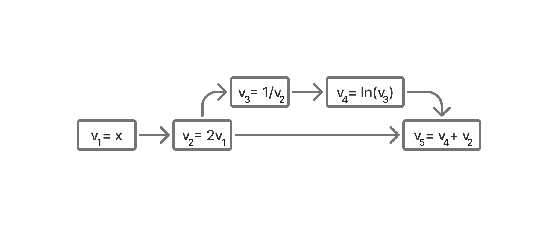
x = Scalar(1.0, "x")
a = x * 2
b = 1 / a
c = b.log()
d = c + a
d
Scalar(value=1.30685, grad=0, name='(ln((1 / (x * 2))) + (x * 2))')
d.backward()
x.grad
1.0
invalid_backward(d)
x.grad   # wrong: a passed on its adjoint to d before c contributed to it
Visiting (ln((1 / (x * 2))) + (x * 2)), adjoint=1
   Propagating to ln((1 / (x * 2))) with local derivative 1
   Propagating to (x * 2) with local derivative 1
Visiting (x * 2), adjoint=1
   Propagating to x with local derivative 2
   Propagating to 2 with local derivative 1
Visiting 2, adjoint=1
Visiting x, adjoint=2
Visiting ln((1 / (x * 2))), adjoint=1
   Propagating to (1 / (x * 2)) with local derivative 2
Visiting (1 / (x * 2)), adjoint=2
   Propagating to 1 with local derivative 0.5
   Propagating to (x * 2) with local derivative -0.25
Visiting 1, adjoint=1
2.0
Backpropagation in Neural Networks
Let's return to our network example from the slides: two inputs, three sigmoid hidden units, a sigmoid output, and no biases. Let's assume one data point $(\mathbf{x}, t)$, so $E_n = -\left[t \ln y + (1 - t)\ln(1 - y)\right]$:
$$ \mathbf{a}^{(1)} = W^{(1)}\mathbf{x}, \qquad \mathbf{z}^{(1)} = \sigma\left(\mathbf{a}^{(1)}\right), \qquad a^{(2)} = W^{(2)}\mathbf{z}^{(1)}, \qquad y = \sigma\left(a^{(2)}\right). $$
One way to perform autodiff is to build the network from our existing Scalars, with one Scalar per weight. backward() can compute the gradient, and we can compare it with derived formulas:
$$ \delta^{(2)} = \frac{\partial E_n}{\partial a^{(2)}} = y-t, \qquad \frac{\partial E_n}{\partial W^{(2)}} = \delta^{(2)}\left(\mathbf{z}^{(1)}\right)^{\mathsf T}, $$
$$ \delta^{(1)} = \frac{\partial E_n}{\partial \mathbf{a}^{(1)}} = \left(W^{(2)}\right)^{\mathsf T}\delta^{(2)} \odot \mathbf{z}^{(1)} \odot \left(1-\mathbf{z}^{(1)}\right), \qquad \frac{\partial E_n}{\partial W^{(1)}} = \delta^{(1)}\mathbf{x}^{\mathsf T}. $$
rng = np.random.default_rng(13)
W1_values = rng.normal(size=(3, 2))     # 3 hidden units, 2 inputs
W2_values = rng.normal(size=(1, 3))
x_in, t = np.array([1.0, 2.0]), 1.0

def error_scalar(W1_values, W2_values):
    """E_n for one data point, built from Scalars; returns (E_n, W1, W2)."""
    W1 = [[Scalar(W1_values[i, j], f"W1[{i},{j}]") for j in range(2)] for i in range(3)]
    W2 = [Scalar(W2_values[0, i], f"W2[{i}]") for i in range(3)]
    z = [sum(W1[i][j] * x_in[j] for j in range(2)).sigmoid() for i in range(3)]
    y = sum(W2[i] * z[i] for i in range(3)).sigmoid()
    E_n = -(t * y.log() + (1 - t) * (1 - y).log())
    return E_n, W1, W2

E_n, W1, W2 = error_scalar(W1_values, W2_values)
E_n.backward()
dW1_graph = np.array([[w.grad for w in row] for row in W1])
dW2_graph = np.array([[w.grad for w in W2]])

# the derived gradient formulas
sigma = lambda a: 1 / (1 + np.exp(-a))
xc = x_in.reshape(2, 1)
z = sigma(W1_values @ xc)
y = sigma(W2_values @ z)
delta2 = y - t
dW2 = delta2 @ z.T
delta1 = (W2_values.T @ delta2) * z * (1 - z)
dW1 = delta1 @ xc.T

print("dE/dW2 (formula):\n", dW2)
print("dE/dW1 (formula):\n", dW1)
print("shapes:", dW1.shape, dW2.shape)
print("max difference, graph vs formula:", np.abs(dW1_graph - dW1).max(), np.abs(dW2_graph - dW2).max())
dE/dW2 (formula):
 [[-0.00781841 -0.45100153 -0.53528641]]
dE/dW1 (formula):
 [[-0.01410057 -0.02820114]
 [-0.00358254 -0.00716508]
 [ 0.03042973  0.06085945]]
shapes: (3, 2) (1, 3)
max difference, graph vs formula: 6.938893903907228e-17 5.551115123125783e-17
Gradient checking (Bishop, Section 8.1.4): we can also compare with the numerical gradient:
def numerical_gradient(values, eps=1e-6):
    """Central difference estimate of dE_n/dW for the weights stored in `values`."""
    grad = np.zeros_like(values)
    for idx in np.ndindex(values.shape):
        old = values[idx]
        values[idx] = old + eps
        e_plus = error_scalar(W1_values, W2_values)[0].value
        values[idx] = old - eps
        e_minus = error_scalar(W1_values, W2_values)[0].value
        values[idx] = old
        grad[idx] = (e_plus - e_minus) / (2 * eps)
    return grad

def rel_error(a, b):
    return np.max(np.abs(a - b) / np.maximum(np.abs(a), np.abs(b)))

print("relative error, graph vs numerical:", rel_error(dW1_graph, numerical_gradient(W1_values)),
      rel_error(dW2_graph, numerical_gradient(W2_values)))
relative error, graph vs numerical: 9.227840777453138e-09 1.5024125420149327e-09
The graph and the formulas agree to machine precision, and the central differences agree to about $10^{-8}$ in relative error, as expected for $\epsilon = 10^{-6}$. Each gradient has the shape of its weight matrix: $3 \times 2$ for $W^{(1)}$ and $1 \times 3$ for $W^{(2)}$.
This is of course one way to handle autodiff for for matrices, but was highly inefficient. We had to hand-design each matrix and operation and we did not take advantage of vectorization speedups offered by linear algebra packages. Your task in Homework 3 Coding Part 1 is to implement a more capable version of autodiff for matrices.